Market Structure and Firm Behavior:
Perfect Competition
Dr. Amy McCormick Diduch
The perfectly competitive market
Firm decision-making is complex, encompassing the choice of output levels, product prices, production techniques and strategies for increasing demand. The firm’s competitive environment has a significant impact on the kinds of choices available to a firm. Thus, economic theory of the firm begins with a close look at the structure of market competition. Firms operating in highly competitive markets face different choices from firms operating in oligopolized markets.
Firm decisions are initially categorized by the time frame needed to enact them. Short run decisions involve factors of production that can be changed relatively quickly whereas long run decisions involve factors of production that take more time to change. In the short run, firms can select different quantities of variable inputs (those that are relatively easy to change, such as raw materials, energy or possibly number of workers) and can then use these inputs to produce a higher or lower quantity of output in response to current market conditions (most notably, price). In the long run, firms can change all of its inputs, including those that are fixed in the short run, such as the size of their facility or the amount of physical capital. New firms can enter an industry in the long run and current firms can exit.
How does a firm determine its “best” (i.e. profit-maximizing) output level in the short run? The answer depends on the kind of competition the firm faces. This tutorial covers the behavior of the idealized firm in the market structure known as perfect competition.
Firms in a perfectly competitive market produce the greatest combined output at the lowest possible price and create the most efficiency for the economy as a whole. Few real markets come close to attaining this competitive ideal, however, because the assumptions behind this market are quite restrictive. The perfectly competitive model is most useful as a point of comparison for the other market structures, as it allows us to calculate the amount of inefficiency introduced by non-competitive markets.
A market is perfectly competitive if:
Since each firm produces a product identical to every other firm’s product and each firm is small relative to the overall size of the market, firms have no ability to influence the market price and must act as price takers.
Why are competitive firms price takers? Imagine if such a firm tried to charge a price higher than the market equilibrium price. Who would buy this firm’s products? If these products are truly identical to those produced by every other firm, the firm would find no buyers. Conversely, would this firm gain any advantage by setting its price below the market equilibrium? No! To understand why, think about the meaning of “market equilibrium” – the price at which the quantity that firms want to supply exactly equals the quantity that consumers want to purchase. If your firm can already sell all that it wants to produce at the current equilibrium price, why would it want to sell this same quantity at a lower price? This would simply bring the firm less total revenue without gaining any long term market advantage.
The graphs below illustrate the market equilibrium price and quantity (on the left) and the firm’s view of this market (on the right). The market supply curve in the graph on the left reflects the desired quantity supplied at any price by all of the many, many firms in the market while the market demand curve in this graph reflects the desired quantity demanded at any price by all of the many, many buyers in the market.
Perfect Competition
Dr. Amy McCormick Diduch
The perfectly competitive market
Firm decision-making is complex, encompassing the choice of output levels, product prices, production techniques and strategies for increasing demand. The firm’s competitive environment has a significant impact on the kinds of choices available to a firm. Thus, economic theory of the firm begins with a close look at the structure of market competition. Firms operating in highly competitive markets face different choices from firms operating in oligopolized markets.
Firm decisions are initially categorized by the time frame needed to enact them. Short run decisions involve factors of production that can be changed relatively quickly whereas long run decisions involve factors of production that take more time to change. In the short run, firms can select different quantities of variable inputs (those that are relatively easy to change, such as raw materials, energy or possibly number of workers) and can then use these inputs to produce a higher or lower quantity of output in response to current market conditions (most notably, price). In the long run, firms can change all of its inputs, including those that are fixed in the short run, such as the size of their facility or the amount of physical capital. New firms can enter an industry in the long run and current firms can exit.
How does a firm determine its “best” (i.e. profit-maximizing) output level in the short run? The answer depends on the kind of competition the firm faces. This tutorial covers the behavior of the idealized firm in the market structure known as perfect competition.
Firms in a perfectly competitive market produce the greatest combined output at the lowest possible price and create the most efficiency for the economy as a whole. Few real markets come close to attaining this competitive ideal, however, because the assumptions behind this market are quite restrictive. The perfectly competitive model is most useful as a point of comparison for the other market structures, as it allows us to calculate the amount of inefficiency introduced by non-competitive markets.
A market is perfectly competitive if:
- There are many, many small firms. (So many firms that a decision by any one individual firm to increase or decrease its output level will be barely noticeable in the market supply curve for the product).
- All of the firms produce identical (i.e. homogeneous) products. There is no reason for any consumer to form a preference for one firm’s product over another.
- It is easy for new firms to enter this market (i.e. start producing output) and for old firms to exit the market (i.e. stop producing output and leave the industry).
- Firms and customers have access to accurate (i.e. perfect) information needed to make good decisions about buying and producing the product.
- Even if all of these conditions are satisfied, a market will not reach its efficient price and quantity if there are negative externalities (such as pollution) or positive externalities (such as societal benefits conveyed by education).
Since each firm produces a product identical to every other firm’s product and each firm is small relative to the overall size of the market, firms have no ability to influence the market price and must act as price takers.
Why are competitive firms price takers? Imagine if such a firm tried to charge a price higher than the market equilibrium price. Who would buy this firm’s products? If these products are truly identical to those produced by every other firm, the firm would find no buyers. Conversely, would this firm gain any advantage by setting its price below the market equilibrium? No! To understand why, think about the meaning of “market equilibrium” – the price at which the quantity that firms want to supply exactly equals the quantity that consumers want to purchase. If your firm can already sell all that it wants to produce at the current equilibrium price, why would it want to sell this same quantity at a lower price? This would simply bring the firm less total revenue without gaining any long term market advantage.
The graphs below illustrate the market equilibrium price and quantity (on the left) and the firm’s view of this market (on the right). The market supply curve in the graph on the left reflects the desired quantity supplied at any price by all of the many, many firms in the market while the market demand curve in this graph reflects the desired quantity demanded at any price by all of the many, many buyers in the market.
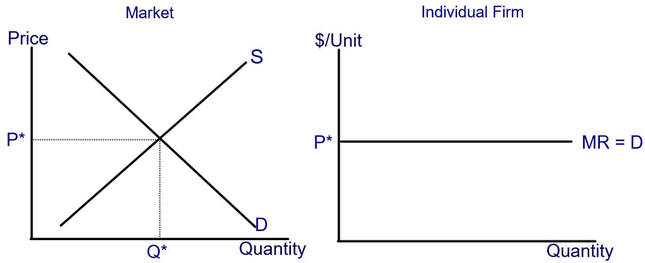
In the graph on the right side, the individual firm observes the market equilibrium price, P*. The firm recognizes that for each additional unit the firm sells, it will receive the market price in exchange. For this reason, the market price is equal to the firm’s marginal revenue (MR), or the change in total revenue received when the firm sells one more unit of output. We could also label this curve as the firm’s demand curve. A horizontal demand curve such as this one illustrates perfectly elastic demand, in which any small increase in price would cause quantity demanded to fall to zero. This is, in fact the situation faced by a firm in a perfectly competitive industry.
The output decision for the perfectly competitive firm
The primary short-run decision for a perfectly competitive firm is to choose its output quantity. Profit-maximization requires that firms produce where the marginal revenue received from the last unit produced just equals the marginal cost of its production. In a perfectly competitive market, a firm’s marginal revenue is equal to the equilibrium market price. Thus, in perfect competition, a firm should choose the output level at which Price = Marginal Cost. The graph below illustrates this decision:
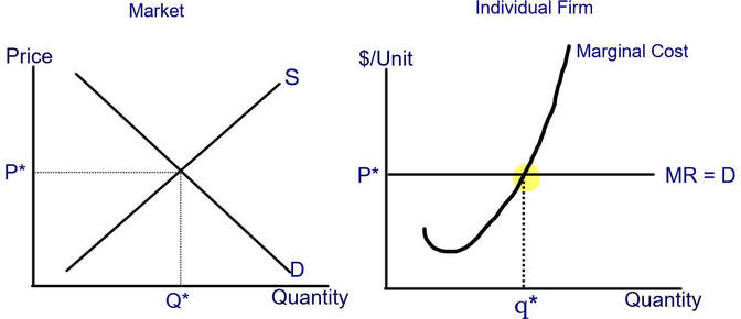
The J-shaped marginal cost curve illustrates the “typical” increments in costs for any firm that faces diminishing marginal product of its inputs in the short run. Profit is maximized at the quantity for which price (which is equivalent to marginal revenue) equals marginal cost. This occurs where the price / marginal revenue / demand curve crosses the marginal cost curve (highlighted in yellow, with the vertical dotted line pointing towards the optimal quantity of output). I’ve chosen to use the lower case q* here to indicate the individual firm’s optimal quantity and the upper case Q* to indicate the market equilibrium quantity (which is the sum of output levels of all firms, or q1 + q2 + q3 + ….).
If we can estimate a firm’s full marginal cost function, we can solve the firm’s profit-maximization problem algebraically. For example, if the market price is $30 and a firm’s marginal costs take the form MC = 10 + 2q, the profit maximizing output can be found by setting P = MC, or $30 = 10 + 2q which solves for a profit-maximizing quantity of 10.
Profits or losses in the short run and long run
Selecting the profit-maximizing quantity of output does not guarantee that the firm is making economic profits. We can use graphs or algebra (or tables with revenue and cost data) to calculate the firm’s profits at its preferred output level. To do so, we need some additional information about the firm’s total and average costs of production.
Profit is defined as Total Revenue – Total Cost. These “total” values are not in “per unit” terms and can’t be sketched on the same graph with the “per unit” values we’ve used in our perfect competition graph. For example, marginal cost is defined as the cost of producing one more unit. Marginal revenue is the extra revenue received from selling one more unit. However, we can transform our calculation of Profit into “per unit” terms as follows:
Profit = Total Revenue – Total Cost
Multiply by one, or Q/Q: Profit = Q/Q * (Total Revenue – Total Cost).
Write Total Revenue as its equation, P*Q: Profit = Q/Q * (P*Q – Total Cost).
Distribute the Q in the denominator throughout the equation: Profit = Q* (P*Q/Q – (Total Cost)/Q).
TC/Q = average total cost, so rewrite as: Profit = Q (P – ATC)
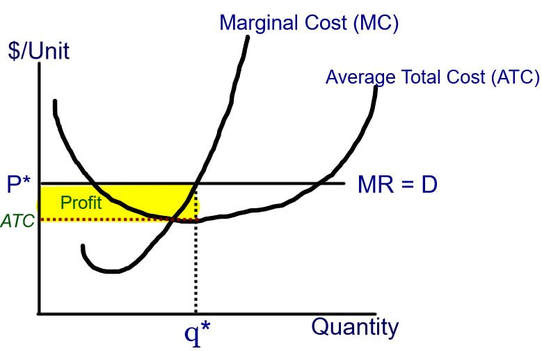
Thus, Profit = Q (P – ATC) and we can easily find this area in a graph. Q is the perfectly competitive level of output (found at the intersection of the marginal cost and marginal revenue (i.e. price) curves. The second part, (P-ATC), is the vertical distance between the market price and the average total cost of producing the competitive output level. The “typical” average total cost curve has a U-shape (again reflecting the eventual problem of diminishing returns to production inputs in the short run). We need to sketch the Average Total Cost curve (ATC) onto our original graph and note the vertical distance between price and ATC at the profit-maximizing level of output.
If we can estimate a firm’s full marginal cost function, we can solve the firm’s profit-maximization problem algebraically. For example, if the market price is $30 and a firm’s marginal costs take the form MC = 10 + 2q, the profit maximizing output can be found by setting P = MC, or $30 = 10 + 2q which solves for a profit-maximizing quantity of 10.
Profits or losses in the short run and long run
Selecting the profit-maximizing quantity of output does not guarantee that the firm is making economic profits. We can use graphs or algebra (or tables with revenue and cost data) to calculate the firm’s profits at its preferred output level. To do so, we need some additional information about the firm’s total and average costs of production.
Profit is defined as Total Revenue – Total Cost. These “total” values are not in “per unit” terms and can’t be sketched on the same graph with the “per unit” values we’ve used in our perfect competition graph. For example, marginal cost is defined as the cost of producing one more unit. Marginal revenue is the extra revenue received from selling one more unit. However, we can transform our calculation of Profit into “per unit” terms as follows:
Profit = Total Revenue – Total Cost
Multiply by one, or Q/Q: Profit = Q/Q * (Total Revenue – Total Cost).
Write Total Revenue as its equation, P*Q: Profit = Q/Q * (P*Q – Total Cost).
Distribute the Q in the denominator throughout the equation: Profit = Q* (P*Q/Q – (Total Cost)/Q).
TC/Q = average total cost, so rewrite as: Profit = Q (P – ATC)
Thus, Profit = Q (P – ATC) and we can easily find this area in a graph. Q is the perfectly competitive level of output (found at the intersection of the marginal cost and marginal revenue (i.e. price) curves. The second part, (P-ATC), is the vertical distance between the market price and the average total cost of producing the competitive output level. The “typical” average total cost curve has a U-shape (again reflecting the eventual problem of diminishing returns to production inputs in the short run). We need to sketch the Average Total Cost curve (ATC) onto our original graph and note the vertical distance between price and ATC at the profit-maximizing level of output.
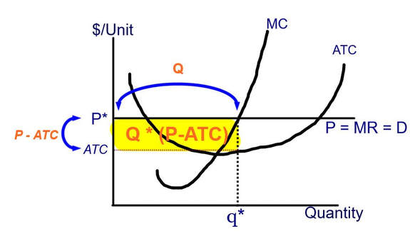
The profit equation, Q * (P-ATC), reflects the length and width of a rectangle, as illustrated in the graph below. Thus, the profit calculation is simply the area of a rectangle bounded by the distance (P-ATC) and Q.
In the above graph, price is greater than average total cost so this firm must be making an economic profit (where revenues exceed both its accounting costs and its opportunity costs). Use the equation for profit to convince yourself this must be true!
Firms may certainly lose money. In the graph below, the equilibrium market price is less than average total cost at the profit-maximizing level of output:
Firms may certainly lose money. In the graph below, the equilibrium market price is less than average total cost at the profit-maximizing level of output:
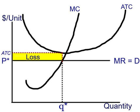
Notice in the graph that at the profit-maximizing output level (q*), the average total cost of production (ATC) is above the equilibrium market price. Again, use the equation to convince yourself that the firm must be losing money when Price is less than Average Total Cost.
Entry and Exit in the Long Run
One of the key insights of the perfectly competitive model is that the relative ease with which new firms can enter the market (and old firms can exit the market) means that market supply – and thus, market price – will change as profit and loss conditions change. When most firms in the industry are making profits, new firms will want to enter this market. As new firms enter, market supply will increase and the equilibrium market price will decrease. As the price falls, firm profits will start falling as well.
Conversely, when most firms are losing money, some will exit the market entirely. As this occurs, the market supply will decrease and the equilibrium market price will begin to increase. The losses experienced by the remaining firms will lessen over time.
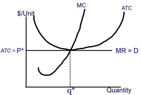
If firm profits attract entry of new firms and firm losses cause exit of existing firms, the long run competitive equilibrium in a perfectly competitive industry must be one in which firms make zero economic profits, as illustrated by the following graph, where average total cost = price = marginal cost at the profit-maximizing level of output:
Entry and Exit in the Long Run
One of the key insights of the perfectly competitive model is that the relative ease with which new firms can enter the market (and old firms can exit the market) means that market supply – and thus, market price – will change as profit and loss conditions change. When most firms in the industry are making profits, new firms will want to enter this market. As new firms enter, market supply will increase and the equilibrium market price will decrease. As the price falls, firm profits will start falling as well.
Conversely, when most firms are losing money, some will exit the market entirely. As this occurs, the market supply will decrease and the equilibrium market price will begin to increase. The losses experienced by the remaining firms will lessen over time.
If firm profits attract entry of new firms and firm losses cause exit of existing firms, the long run competitive equilibrium in a perfectly competitive industry must be one in which firms make zero economic profits, as illustrated by the following graph, where average total cost = price = marginal cost at the profit-maximizing level of output:
Although entry and exit of firms drive profits towards zero in the long run, firms may find themselves with tough decisions in the short run before market prices have time to adjust. When a firm is losing money in the short run, is it better off producing q* or should it shut down? The answer depends on the firm’s mixture of fixed and variable costs. Variable costs are those associated with a particular output level: to increase output, you need to use more of your variable inputs, so those costs increase. To decrease output, you use less of your variable inputs, so those costs decrease. If you decrease your output to zero (i.e. shut down your production), your variable costs decrease to zero. Fixed costs (such as loan payments or rent on a building) do not vary with your production level. If you shut down production in the short run, you still face the problem of how to pay your fixed costs (at least until you exit the industry, which can occur in the longer run only after finding a way to dispose of your remaining fixed costs).
Thus, the general rule of thumb is to keep producing, despite short run losses, as long as price is high enough to cover your per-unit variable costs of production and possibly allow you to pay something towards your fixed costs. Mathematically, you are comparing two options: your profits if you produce q* (calculated as Total Revenue – Total Variable Cost – Total Fixed Cost) and your profits if you shut down and produce nothing (calculated as – Fixed Costs, since you have zero revenue and zero variable costs).
Thus, the firm will produce q* as long as (TR – VC) – FC ≥ – FC
Adding FC to both sides (TR – VC) ≥ (-FC) + FC
Results in (TR – VC) ≥ 0
Multiplying both sides by 1/Q, TR/Q – VC/Q ≥ 0
TR/Q = P, VC/Q = AVC P – AVC ≥ 0
Rearranging, P ≥ AVC
Thus, our rule of thumb says that as long as Price is greater than Average Variable Cost, the firm makes smaller losses by continuing to produce at the profit-maximizing level of output. However, if Price falls below Average Variable Cost, the firm is better off shutting down and producing 0. In this case, the firm still needs to find a way to pay its Fixed Costs but it won’t incur even larger losses from using variable inputs that it cannot pay for.
Thus, the rule for a firm that is losing money:
Produce q* when P≥AVC
Shut down and set q=0 when P<AVC
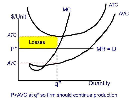
The graph below illustrates the situation in which a firm should continue to produce despite losses:
Thus, the general rule of thumb is to keep producing, despite short run losses, as long as price is high enough to cover your per-unit variable costs of production and possibly allow you to pay something towards your fixed costs. Mathematically, you are comparing two options: your profits if you produce q* (calculated as Total Revenue – Total Variable Cost – Total Fixed Cost) and your profits if you shut down and produce nothing (calculated as – Fixed Costs, since you have zero revenue and zero variable costs).
Thus, the firm will produce q* as long as (TR – VC) – FC ≥ – FC
Adding FC to both sides (TR – VC) ≥ (-FC) + FC
Results in (TR – VC) ≥ 0
Multiplying both sides by 1/Q, TR/Q – VC/Q ≥ 0
TR/Q = P, VC/Q = AVC P – AVC ≥ 0
Rearranging, P ≥ AVC
Thus, our rule of thumb says that as long as Price is greater than Average Variable Cost, the firm makes smaller losses by continuing to produce at the profit-maximizing level of output. However, if Price falls below Average Variable Cost, the firm is better off shutting down and producing 0. In this case, the firm still needs to find a way to pay its Fixed Costs but it won’t incur even larger losses from using variable inputs that it cannot pay for.
Thus, the rule for a firm that is losing money:
Produce q* when P≥AVC
Shut down and set q=0 when P<AVC
The graph below illustrates the situation in which a firm should continue to produce despite losses:
Calculating profits and losses using algebra
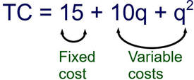
The information conveyed by the perfect competition graphs can be expressed in equation form. At a minimum, we need to know the market price and the total cost function. We’ll use the marginal cost function introduced earlier in this tutorial, MC = 10 + 2q, and the Total Cost function TC = 15 + 10q + q2. (If you know calculus, you can take the first derivative with respect to q of this Total Cost function and will find that it equals 10 + 2q). Let’s look at the cost relationships we can derive from this information before moving on to the profit-maximization problem.
In the short run, firms face both fixed costs and variable costs. The total cost function provides information on both of these cost categories. Variable costs are those that change as the level of output changes (so they will be multiples of the quantity of output, q). Fixed costs are those that do not change when output changes. For the total cost function above,
The other cost curves can be calculated as follows:
Average Total Cost (ATC) = TC/q = (15 + 10q + q2)/q = 15/q + 10 + q.
Average Variable Cost (AVC) = TVC/q = (10q + q2) / q = 10 + q.
Assume, again, that the market price is $30. What do these equations tell us about the firm’s decisions?
Step 1: Find the profit-maximizing output level by setting P = MC and solving for q:
P = MC
30 = 10 + 2q
20 = 2q
10 = q
Step 2: Find profit (π)
We can do using either equation. We can calculate π = Q * (P- ATC) or we can calculate π = TR – TC
We know q and we know P. What is ATC when q = 10? Plug q=10 into the ATC equation:
ATC = 15/q + 10 + q
ATC = 15/10 + 10 + 10 = 21.5
Therefore, π = Q * (P- ATC) = 10 * (30 – 21.5) = $85
Alternatively, π = TR – TC
TR = P * Q = $30 * 10 = $300
TC = 15 + 10q + q2 = 15 + 10*(10) + 102 = 15 + 100 + 100 = $215
π = TR – TC = $300 - $215 = $85
Suppose market conditions change and this firm now faces a market price of $15. How does this affect the firm’s output level and profits?
Step 1: Find the profit-maximizing output level by setting P = MC and solving for q:
P = MC
15 = 10 + 2q
5 = 2q
2.5 = q
Step 2: Find profit. Let’s calculate it as π = TR – TC
TR = P * Q = $15*2.5 = 37.5
TC = 15 + 10q + q2 = 15 + 10(2.5) + (2.5)2 = 15+25+6.25=46.25
37.5 - 46.25= – $8.75
This firm is losing money! Is it better off producing 2.5 units and losing $8.75 or should this firm shut down and set q=0? Our rule of thumb says to produce q* as long as P> AVC. What is AVC when q = 2.5? Plug q=2.5 into the equation for AVC (above):
AVC = 10 + q = 10 + 2.5 = 12.5. Price is $15 and AVC is 12.5, so this firm should continue to produce 2.5 units of output.
Check to see that the firm loses less by producing at q = 2.5 than if it shuts down and produces q= 0:
Losses when q = 2.5 are -$8.75
Losses if the firm shuts down and produces q = 0 equal the firm’s fixed costs of $15.
Thus, this firm IS better off producing q = 2.5 rather than shutting down and producing q = 0.
Problem solving using tables:
Econ 101 textbooks frequently present firm cost and price information in table form. This requires students to know (and possibly calculate) the various cost relationships and then be able to apply the decision rule, in which firms choose output where P = MC. Profit can then be calculated as TR – TC or as Q*(P-ATC) depending on the information already present in the table.
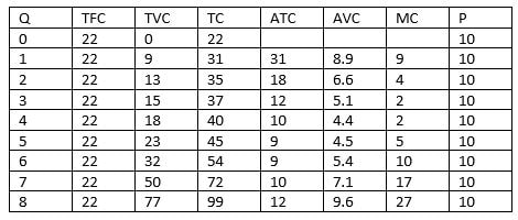
The table below presents the full set of cost information for a firm. You can check to see that these values add up. For example, we know that Total Cost (TC) is the sum of fixed and variable costs (TFC and TVC). We don’t really need the fixed cost column: we can find its value either by subtracting the variable costs from the total costs or by checking on the value of Total Cost when quantity is zero (and thus the firm has no variable costs).
You can also check the average and marginal cost values. Average Total Cost (ATC) is Total Cost divided by quantity. Average variable cost is Total Variable Cost divided by quantity. Marginal cost is the change in Total cost resulting from a one-unit increase in output. This firm should produce where Price = Marginal Cost; by choosing an output quantity of 6, this firm will earn total revenue of 6*$10 = $60 and face total costs of $54, earning a profit of $6.
The file below contains practice problems for perfect competition.
| practice_problems_for_perfect_competition.pdf |
Want to see these concepts demonstrated step-by-step? The videos below cover the perfectly competitive model.
