Price Elasticity of Demand (with a few notes on Price Elasticity of Supply)
Dr. Amy McCormick Diduch
Elasticity is a measure of responsiveness to a change. Elasticity values can help firms decide how to set prices or help governments decide which goods or services to tax. This tutorial covers the calculation of price elasticity of demand; however, there are many other elasticity calculations that are highly useful to economic analysis.
Price elasticity of demand measures the responsiveness of quantity demanded to a change in price. Quantity demanded is highly elastic if it changes dramatically in response to a price change. (Highly elastic demand is like a very stretchy rubber band – it can easily change position). Quantity demanded is highly inelastic if it changes very little in response to a price change. (Highly inelastic demand is like a very stiff rubber band – it is hard to change its position very much).
1. Calculating elasticity of demand
It doesn’t take too much searching to find newspaper articles that contain a statement such as “diamond prices rose 15% last year, resulting in a 10% decline in net sales.” Assuming that the price increase is the only reason for the decline in quantity demanded, we can use these figures to calculate the price elasticity of demand, which tells us whether the change in quantity demanded was “large” or “small” in importance.
Price elasticity of demand = ED = % change in quantity demanded
% change in price
(Or, price elasticity of demand = percentage change in quantity demanded DIVIDED BY percentage change in price).
For the hypothetical diamond example above, the price elasticity of demand would be:
ED = -10% change in quantity demanded / 15% change in price = │-0.67│ = 0.67
(Note that I’ve expressed this result in absolute value terms. The negative sign reflects the negative relationship between price and quantity along a demand curve. It doesn’t provide us with additional useful information in this example so we are safe to ignore it and use the absolute value).
How do we interpret the resulting value? In our diamond example, notice that the percentage change in price was larger than the resulting percentage change in quantity demanded. In other words, the size of the quantity response was small relative to the size of the price change, resulting in an elasticity value less than 1.
Demand is described as inelastic if the price elasticity of demand is less than 1. Inelastic demand indicates the change in quantity demanded is small relative to the change in price.
Inelastic demand = SMALLER % change in quantity demanded
LARGER % change in price
Goods and services that are likely to have inelastic demand are those that (1) have very few good substitutes, (2) are considered to be necessities, (3) take a very small share of the consumer’s budget or (4) the consumer has very little time to adjust behavior in response to the price change.
Demand is described as elastic if the price elasticity of demand is greater than 1. Elastic demand indicates the change in quantity demanded is large relative to the change in price.
Elastic demand = LARGER % change in quantity demanded
SMALLER % change in price
Goods and services that are likely have elastic demand are those that (1) have many good substitutes (including competing brands of the product), (2) are considered to be luxuries, (3) take a fairly large share of the consumer’s budget or (4) products for which the consumer has plenty of time to adjust their behavior in response to the price change.
Demand is described as unit elastic if the price elasticity of demand equals 1.
Suppose price increased by 15% but quantity demanded did not change at all?
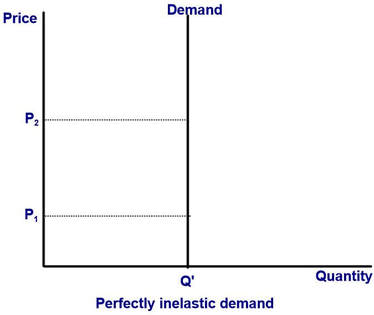
In this case the price elasticity of demand would be 0%/15% = 0; we describe this as perfectly inelastic demand. Here, price doesn’t matter to the consumer: they will continue to purchase their desired amount even when prices change significantly. The graph below illustrates a perfectly inelastic demand curve: if price increases from P1 to P2, quantity demanded does not change at all. Demand will be perfectly inelastic (or close to perfectly inelastic) for goods that are considered to be necessities.
Dr. Amy McCormick Diduch
Elasticity is a measure of responsiveness to a change. Elasticity values can help firms decide how to set prices or help governments decide which goods or services to tax. This tutorial covers the calculation of price elasticity of demand; however, there are many other elasticity calculations that are highly useful to economic analysis.
Price elasticity of demand measures the responsiveness of quantity demanded to a change in price. Quantity demanded is highly elastic if it changes dramatically in response to a price change. (Highly elastic demand is like a very stretchy rubber band – it can easily change position). Quantity demanded is highly inelastic if it changes very little in response to a price change. (Highly inelastic demand is like a very stiff rubber band – it is hard to change its position very much).
1. Calculating elasticity of demand
It doesn’t take too much searching to find newspaper articles that contain a statement such as “diamond prices rose 15% last year, resulting in a 10% decline in net sales.” Assuming that the price increase is the only reason for the decline in quantity demanded, we can use these figures to calculate the price elasticity of demand, which tells us whether the change in quantity demanded was “large” or “small” in importance.
Price elasticity of demand = ED = % change in quantity demanded
% change in price
(Or, price elasticity of demand = percentage change in quantity demanded DIVIDED BY percentage change in price).
For the hypothetical diamond example above, the price elasticity of demand would be:
ED = -10% change in quantity demanded / 15% change in price = │-0.67│ = 0.67
(Note that I’ve expressed this result in absolute value terms. The negative sign reflects the negative relationship between price and quantity along a demand curve. It doesn’t provide us with additional useful information in this example so we are safe to ignore it and use the absolute value).
How do we interpret the resulting value? In our diamond example, notice that the percentage change in price was larger than the resulting percentage change in quantity demanded. In other words, the size of the quantity response was small relative to the size of the price change, resulting in an elasticity value less than 1.
Demand is described as inelastic if the price elasticity of demand is less than 1. Inelastic demand indicates the change in quantity demanded is small relative to the change in price.
Inelastic demand = SMALLER % change in quantity demanded
LARGER % change in price
Goods and services that are likely to have inelastic demand are those that (1) have very few good substitutes, (2) are considered to be necessities, (3) take a very small share of the consumer’s budget or (4) the consumer has very little time to adjust behavior in response to the price change.
Demand is described as elastic if the price elasticity of demand is greater than 1. Elastic demand indicates the change in quantity demanded is large relative to the change in price.
Elastic demand = LARGER % change in quantity demanded
SMALLER % change in price
Goods and services that are likely have elastic demand are those that (1) have many good substitutes (including competing brands of the product), (2) are considered to be luxuries, (3) take a fairly large share of the consumer’s budget or (4) products for which the consumer has plenty of time to adjust their behavior in response to the price change.
Demand is described as unit elastic if the price elasticity of demand equals 1.
Suppose price increased by 15% but quantity demanded did not change at all?
In this case the price elasticity of demand would be 0%/15% = 0; we describe this as perfectly inelastic demand. Here, price doesn’t matter to the consumer: they will continue to purchase their desired amount even when prices change significantly. The graph below illustrates a perfectly inelastic demand curve: if price increases from P1 to P2, quantity demanded does not change at all. Demand will be perfectly inelastic (or close to perfectly inelastic) for goods that are considered to be necessities.
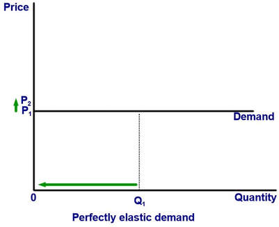
Suppose price increased by a very small amount (say, 0.1%) and quantity demanded decreased by a very large amount (say, 99.9%). Demand is nearly perfectly elastic in this instance. Price is the only thing that matters; if price increases at all, people choose not to buy the product (or switch to competitor brands).
Other examples:
Suppose that a 13% increase in the price of electricity results in a 5% decline in electricity usage. The price elasticity of demand would be │-5% / 13%│ = 0.345, which is inelastic.
Suppose that a 5% decrease in the price of admission to an amusement park resulted in a 17% increase in park attendance. The price elasticity of demand would be │17% / - 5%│ = 3.4, which is elastic.
Suppose that a 9% decrease in the price of roller skates resulted in a 9% increase in sales.
The price elasticity of demand would be│ 9 % / -9 %│ = 1.0, which is unit elastic.
2. Point elasticity of demand
If you know the demand schedule for a product (or have an equation for the demand curve), you can calculate elasticity values for any price and quantity combination along the demand curve using one of two formulas: point elasticity or arc elasticity. If the demand curve is a straight line, the point elasticity calculation is simple and more precise. It requires two steps:
Step 1: calculate the slope of the demand curve.
Step 2: For any given price and quantity combination along this demand curve, calculate the following:
ED = Price elasticity of demand = │ 1/slope │ * P/Q
This is known as the point elasticity formula. We’ll use the absolute value of the inverse of the slope.
(As a side note, the formula derived directly from the definition of price elasticity of demand, which can be written as ∆Q/Q / ∆P/P. This is a fraction divided by a fraction; rearrange to get ∆Q/Q * P/∆P. Rearrange again to get ∆Q/∆P * P/Q or 1/slope * P/Q).
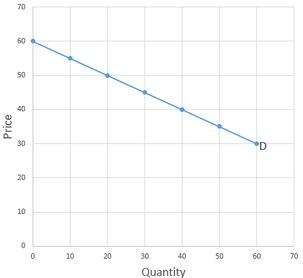
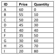
We’ll demonstrate with the following demand schedule (which can be represented by the linear equation P = 60- ½ Q).
Suppose that a 13% increase in the price of electricity results in a 5% decline in electricity usage. The price elasticity of demand would be │-5% / 13%│ = 0.345, which is inelastic.
Suppose that a 5% decrease in the price of admission to an amusement park resulted in a 17% increase in park attendance. The price elasticity of demand would be │17% / - 5%│ = 3.4, which is elastic.
Suppose that a 9% decrease in the price of roller skates resulted in a 9% increase in sales.
The price elasticity of demand would be│ 9 % / -9 %│ = 1.0, which is unit elastic.
2. Point elasticity of demand
If you know the demand schedule for a product (or have an equation for the demand curve), you can calculate elasticity values for any price and quantity combination along the demand curve using one of two formulas: point elasticity or arc elasticity. If the demand curve is a straight line, the point elasticity calculation is simple and more precise. It requires two steps:
Step 1: calculate the slope of the demand curve.
Step 2: For any given price and quantity combination along this demand curve, calculate the following:
ED = Price elasticity of demand = │ 1/slope │ * P/Q
This is known as the point elasticity formula. We’ll use the absolute value of the inverse of the slope.
(As a side note, the formula derived directly from the definition of price elasticity of demand, which can be written as ∆Q/Q / ∆P/P. This is a fraction divided by a fraction; rearrange to get ∆Q/Q * P/∆P. Rearrange again to get ∆Q/∆P * P/Q or 1/slope * P/Q).
We’ll demonstrate with the following demand schedule (which can be represented by the linear equation P = 60- ½ Q).
|
|
First, find the slope of this line and then find its inverse.
Slope is calculated as (change in value along y-axis) / (change in value along x-axis) or “rise” / “run” and can be calculated between any two points on a straight line. Suppose we want to calculate slope between points A and B. Price declines from 60 to 55 when we move from A to B, so the change along the y-axis is -5. Quantity increases from 0 to 10 so the change along the x-axis is 10. The slope from A to B, then, is -5 / 10 = -1/2. (We’ll use the absolute value of this).
Notice that when we already have the equation for the line (in the form y = b + mx or, here, P = 60 - ½ QD), we can read the slope directly from the equation.
The inverse of the slope is just 1/slope or 1 / (½) = 2.
So for this example, the point elasticity formula is ED = 2 * P/Q
An important detail: the slope of this demand curve is constant (and therefore the inverse of the slope is constant) but the price elasticity of demand will be different at each price and quantity combination.
Second, choose a price and quantity combination and calculate price elasticity of demand:
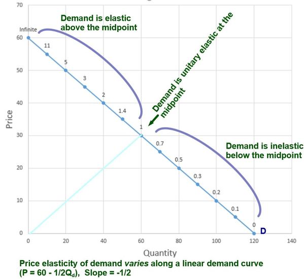
As we move along the demand curve from high prices to low prices, the elasticity value gets smaller and smaller. We will find this relationship along any downward-sloping linear demand curve. The graph below illustrates the entire demand curve (from the equation P = 60 – ½ QD). The numbers given above the demand curve are the elasticity calculations for these price and quantity combinations. Details to notice: (1) demand is elastic at higher prices and becomes more inelastic as prices fall and (2) demand is unit elastic at the midpoint of a downward-sloping linear demand curve.
Thus, even if we know a good is a luxury, say, we can’t be certain that it has elastic demand. The exact elasticity value will depend on its current price.
Slope is calculated as (change in value along y-axis) / (change in value along x-axis) or “rise” / “run” and can be calculated between any two points on a straight line. Suppose we want to calculate slope between points A and B. Price declines from 60 to 55 when we move from A to B, so the change along the y-axis is -5. Quantity increases from 0 to 10 so the change along the x-axis is 10. The slope from A to B, then, is -5 / 10 = -1/2. (We’ll use the absolute value of this).
Notice that when we already have the equation for the line (in the form y = b + mx or, here, P = 60 - ½ QD), we can read the slope directly from the equation.
The inverse of the slope is just 1/slope or 1 / (½) = 2.
So for this example, the point elasticity formula is ED = 2 * P/Q
An important detail: the slope of this demand curve is constant (and therefore the inverse of the slope is constant) but the price elasticity of demand will be different at each price and quantity combination.
Second, choose a price and quantity combination and calculate price elasticity of demand:
- When price is $55, quantity demanded is 10. ED = │1/slope│ * P/Q = 2 * 55/10 = 110/10 = 11, which reflects very elastic demand at this price.
- When price is $40, quantity demanded is 40. ED = │1/slope│ * P/Q = 2 * 40/40 = 2, which is elastic demand.
- When price is $30, quantity demanded is 60. ED = │1/slope│ * P/Q = 2 *30/60 = 1, which is unitary elastic.
- When price is $20, quantity demanded is 80. ED = │1/slope│ * P/Q = 2 *20/80 = ½ or 0.5, which reflects inelastic demand.
As we move along the demand curve from high prices to low prices, the elasticity value gets smaller and smaller. We will find this relationship along any downward-sloping linear demand curve. The graph below illustrates the entire demand curve (from the equation P = 60 – ½ QD). The numbers given above the demand curve are the elasticity calculations for these price and quantity combinations. Details to notice: (1) demand is elastic at higher prices and becomes more inelastic as prices fall and (2) demand is unit elastic at the midpoint of a downward-sloping linear demand curve.
Thus, even if we know a good is a luxury, say, we can’t be certain that it has elastic demand. The exact elasticity value will depend on its current price.
3. Arc elasticity of demand
Suppose we do not have information about the entire demand curve relationship or cannot determine the slope at a particular price and quantity combination. We can still calculate an approximate elasticity value if we know the starting and ending price and quantity combinations.
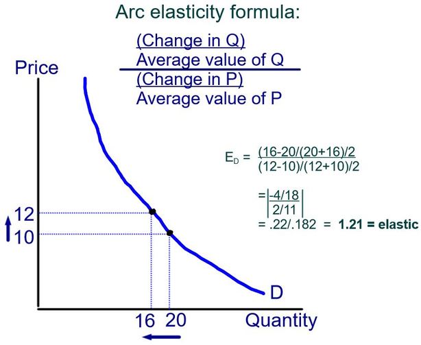
The arc elasticity formula requires a few steps (none of which is mathematically difficult) and is illustrated in the graph below.
Suppose that price increases from $10 to $12, causing quantity to fall from 20 to 16.
- Calculate the percentage change in quantity as (Q2 – Q1) / (Q2 + Q1)/2 (which is the change in Q divided by the average value of Q).
- Calculate the percentage change in price as (P2 – P1) / (P2 + P1)/2 (which is the change in P divided by the average value of P).
- Divide the percentage change in quantity by the percentage change in price. Interpret the result according to whether the value is greater than, less than or equal to 1.
4. Elasticity and total revenue
Suppose you have the following information about the demand schedule for yoga classes (from the first two columns in the table below).
Suppose you have the following information about the demand schedule for yoga classes (from the first two columns in the table below).
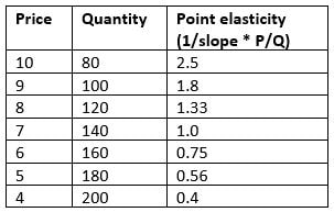
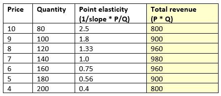
The third column of this table provides the price elasticity of demand at each of the possible prices. (To calculate elasticity: the slope of this demand curve is 1/20. Therefore, to calculate the point elasticity, you take 1/ slope, which equals 20, and multiply it by P/Q. When price is 10, P/Q is 1/8. Multiply by 20 to get the elasticity value of 2.5 given in the third column).
The total revenue earned by a business is equal to the price charged for the good or service multiplied by the quantity sold at that price. If a business knows (at least roughly) the demand schedule for its product, it can estimate the total revenue it would earn for any price it might choose.
The total revenue earned by a business is equal to the price charged for the good or service multiplied by the quantity sold at that price. If a business knows (at least roughly) the demand schedule for its product, it can estimate the total revenue it would earn for any price it might choose.
As it turns out, a business doesn’t have to know its demand schedule exactly to be able to figure out how a price increase or decrease would affect its total revenue. A reasonable estimate of price elasticity of demand at the current price level will provide this information. (By the way, this is one of the many reasons why knowledge of economics is helpful to business managers! A good manager, however, will not simply seek to maximize total revenue. She must take costs into consideration as well.)
The same information is useful for government policy decisions. Knowing whether demand is elastic or inelastic will allow policymakers to estimate, for example, the effect of a change in an entrance fee or toll on the total revenue received by the government.
Here are the important relationships:
Suppose that the current price of the membership is $5 and you know the price elasticity of demand is inelastic (at 0.56). With just this information, you know that if you increase price you will also increase total revenue.
If you are currently charging a price of $7 and find the price elasticity of demand to be 1.0, you know that making small changes in price will not significantly change total revenue.
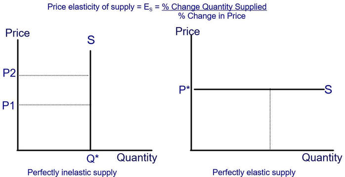
5. Price elasticity of supply
Although there is (generally) a positive relationship between quantity supplied and price, the extent to which quantity supplied increases in response to a price change varies with the amount of time available and the degree to which suppliers have flexibility in production.
Price elasticity of supply is calculated using the same tools as price elasticity of demand. (The point and arc formulas work for supply curves the same way they do for demand curves). Elasticity values are still described as inelastic (for values less than 1) or elastic (for values greater than 1).
Supply will be perfectly inelastic when it is not possible to change the quantity supplied. (An example would be the number of seats in a basketball arena). Supply will be perfectly elastic when a supplier is content to supply any quantity needed at the going price but would not supply any of the product if price were to fall. The diagrams below illustrate these two extremes.
The same information is useful for government policy decisions. Knowing whether demand is elastic or inelastic will allow policymakers to estimate, for example, the effect of a change in an entrance fee or toll on the total revenue received by the government.
Here are the important relationships:
- When demand is elastic, a price increase will result in a reduction in total revenue and a price decrease will result in an increase in total revenue. WHY? Because elastic demand indicates that people change their quantity demanded significantly in response to a price change. When price goes up, they buy a lot less of the product, so total revenue goes down. When price goes down, they buy a lot more of the product, so total revenue goes up.
- When demand is inelastic, a price increase will result in an increase in total revenue and a price decrease will result in a decrease in total revenue. WHY? Because inelastic demand indicates that people do not change quantity demanded significantly in response to a price change. Thus, when price goes up, people don’t reduce quantity demanded by much at all, so total revenue goes up. When price goes down, people don’t increase quantity demanded very much, so total revenue goes down.
Suppose that the current price of the membership is $5 and you know the price elasticity of demand is inelastic (at 0.56). With just this information, you know that if you increase price you will also increase total revenue.
- When demand is unit elastic, a price change will have no impact on total revenue. WHY? Because unit elastic means that the % change in quantity demanded exactly matches the % change in price so the product of (price * quantity) remains the same.
If you are currently charging a price of $7 and find the price elasticity of demand to be 1.0, you know that making small changes in price will not significantly change total revenue.
5. Price elasticity of supply
Although there is (generally) a positive relationship between quantity supplied and price, the extent to which quantity supplied increases in response to a price change varies with the amount of time available and the degree to which suppliers have flexibility in production.
Price elasticity of supply is calculated using the same tools as price elasticity of demand. (The point and arc formulas work for supply curves the same way they do for demand curves). Elasticity values are still described as inelastic (for values less than 1) or elastic (for values greater than 1).
Supply will be perfectly inelastic when it is not possible to change the quantity supplied. (An example would be the number of seats in a basketball arena). Supply will be perfectly elastic when a supplier is content to supply any quantity needed at the going price but would not supply any of the product if price were to fall. The diagrams below illustrate these two extremes.
The file below contains practice problems on elasticity.
| practice_problems_for_price_elasticity_of_demand.pdf |
Want to see step-by-step demonstrations of these concepts? These videos cover the same material:
