Output and price decisions for a monopolist
Dr. Amy McCormick Diduch
A firm with true monopoly power is the only seller of a good or service in its product market. A firm might become a monopolist because it is the first one to create a new good or service. However, the firm will only retain its monopoly status if other firms cannot enter the market to compete against it. These barriers to entry (such as patent laws, sole ownership of a key production resource, or economies of scale that lead to extraordinarily low average production costs) allow the firm to charge a monopoly price – and (potentially) make profits -- for an extended period.
We begin by assuming the firm charges all customers the same price. This simplifies the problem: choose the price / output combination that maximizes the firm’s profits. (More complex models include versions of “price discrimination,” in which the monopolist charges different prices to different customers for the same product. Price discrimination can significantly increase profits but requires more information about customers’ willingness-to-pay for the good).
The monopolist's decision here is an application of marginal analysis: the firm should pursue an action as long as the marginal benefits of doing so are greater than or equal to its marginal costs. A monopolist should produce output up to the point where the marginal revenue of the last unit of output produced is just equal to the marginal cost of producing it (i.e. choose Q where MR=MC). Once the optimal output level is chosen, the monopolist uses information from the demand curve for the product to select its optimal price. Thus, to predict output and price, we need information about the demand curve for the monopolist’s product and the monopolist’s cost structure.
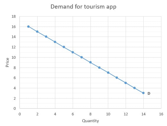
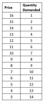
Assume our monopolist is the only seller of a phone app that provides local tourist information. The demand curve for this app is provided in the graph and table below:
Dr. Amy McCormick Diduch
A firm with true monopoly power is the only seller of a good or service in its product market. A firm might become a monopolist because it is the first one to create a new good or service. However, the firm will only retain its monopoly status if other firms cannot enter the market to compete against it. These barriers to entry (such as patent laws, sole ownership of a key production resource, or economies of scale that lead to extraordinarily low average production costs) allow the firm to charge a monopoly price – and (potentially) make profits -- for an extended period.
We begin by assuming the firm charges all customers the same price. This simplifies the problem: choose the price / output combination that maximizes the firm’s profits. (More complex models include versions of “price discrimination,” in which the monopolist charges different prices to different customers for the same product. Price discrimination can significantly increase profits but requires more information about customers’ willingness-to-pay for the good).
The monopolist's decision here is an application of marginal analysis: the firm should pursue an action as long as the marginal benefits of doing so are greater than or equal to its marginal costs. A monopolist should produce output up to the point where the marginal revenue of the last unit of output produced is just equal to the marginal cost of producing it (i.e. choose Q where MR=MC). Once the optimal output level is chosen, the monopolist uses information from the demand curve for the product to select its optimal price. Thus, to predict output and price, we need information about the demand curve for the monopolist’s product and the monopolist’s cost structure.
Assume our monopolist is the only seller of a phone app that provides local tourist information. The demand curve for this app is provided in the graph and table below:
|
|
Suppose the monopolist is currently selling 5 app downloads per day at a price of $12. What is the marginal revenue of selling one more app download per day?
If the monopolist wants to sell 6 app downloads per day, it cannot keep charging a price of $12 per download. The graph and table show that the firm will have to lower the app price to $11. The advantage of this price decrease is that the firm now sells 6 apps per day. The disadvantage is that it gives up the extra $1 in revenue that it used to make on each of the 5 apps per day it previously sold at $12. Selling 5 apps earns the firm $60 in total revenue while selling 6 apps earns $66; thus, total revenue increases by $6. Note that this is less than the price of the tourist app. The 6th app download does sell for $11 but by giving up $1 on each of the 5 apps it previously sold for $12, the extra revenue from selling the 6th app is $11 - $5 or only $6. Our first lesson in monopoly: the marginal revenue from selling an extra unit of output is less than the price of the output (i.e. MR < P).
Marginal revenue is the change in total revenue from selling more unit of output. MR = ∆TR/∆Q.
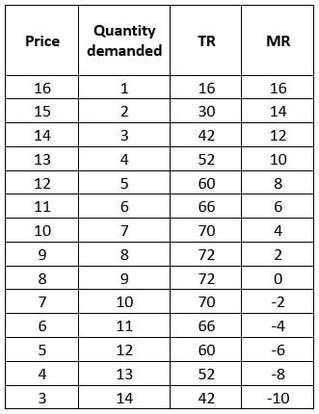
Calculate marginal revenue from the demand curve by first calculating total revenue (TR = P * Q) and then calculating the change in TR for a given change in output, as shown below. (In this example, output always increases by 1 unit). The Total Revenue from selling 4 app downloads is 4*$13 = $52. The Total Revenue from selling 5 app downloads is 5*$12 = $60. The marginal revenue of the 5th app sale per day is $60 - $52 = $8.
If the monopolist wants to sell 6 app downloads per day, it cannot keep charging a price of $12 per download. The graph and table show that the firm will have to lower the app price to $11. The advantage of this price decrease is that the firm now sells 6 apps per day. The disadvantage is that it gives up the extra $1 in revenue that it used to make on each of the 5 apps per day it previously sold at $12. Selling 5 apps earns the firm $60 in total revenue while selling 6 apps earns $66; thus, total revenue increases by $6. Note that this is less than the price of the tourist app. The 6th app download does sell for $11 but by giving up $1 on each of the 5 apps it previously sold for $12, the extra revenue from selling the 6th app is $11 - $5 or only $6. Our first lesson in monopoly: the marginal revenue from selling an extra unit of output is less than the price of the output (i.e. MR < P).
Marginal revenue is the change in total revenue from selling more unit of output. MR = ∆TR/∆Q.
Calculate marginal revenue from the demand curve by first calculating total revenue (TR = P * Q) and then calculating the change in TR for a given change in output, as shown below. (In this example, output always increases by 1 unit). The Total Revenue from selling 4 app downloads is 4*$13 = $52. The Total Revenue from selling 5 app downloads is 5*$12 = $60. The marginal revenue of the 5th app sale per day is $60 - $52 = $8.
|
|
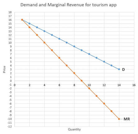
Marginal revenue is always less than price (except for the first unit sold). Marginal revenue can also be negative! Suppose the firm has set a price of $8 (selling 9 units). What is the marginal revenue of selling the 10th app download per day? Total revenue would fall from $72 to $70 so the marginal revenue of the 10th download is -$2.
An important detail that can help with sketching and solving monopoly problems: when the demand curve has a constant slope (like this one, which has a slope of -1), the marginal revenue curve will have a slope exactly twice as steep (here, a slope of -2). Marginal revenue will be 0 when demand is unit elastic. MR>0 when demand is elastic and MR<0 when demand is inelastic.
A savvy monopolist doesn’t simply try to maximize revenue. Profits are greatest when marginal benefits are equal to marginal costs. We know how to calculate the monopolist’s marginal revenue; now we add information about the firm’s cost structure to determine the optimal output level. The table below presents this firm’s total, average and marginal costs of production (as well as profits):
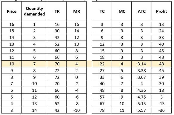
The firm maximizes profits when it sets Marginal Revenue equal to Marginal Cost. According to the table above (and the graph below), this occurs at a quantity of 7. The firm sets the price at $10 per download and makes a profit of $48 per day. (Presenting data in this table form makes it seem like a price of $11 is also profit-maximizing. The use of algebra – rather than a table – to problem-solve would help us distinguish between these two choices).
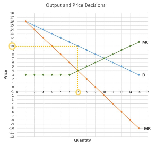
The graph of the monopolist’s decision is more complex than the graph for perfect competition. The key is to focus on the process: (1) find the optimal quantity of output where MR = MC (where the green MC and orange MR lines cross in the graph above) then (2) Use the demand curve (the blue line in the graph above) to identify the optimal price associated with the optimal quantity. (At a quantity of seven, the demand curve shows us the firm can charge a price of $10).
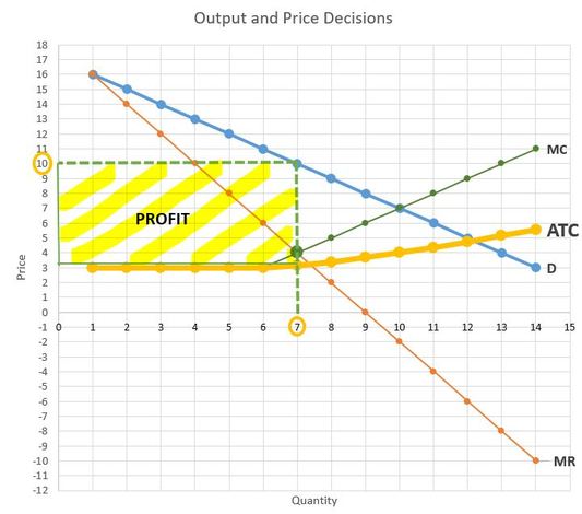
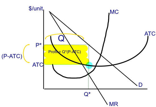
The third step, determining the firm’s profit or loss, requires the addition of the firm’s Average Total Cost curve to the graph. Profit is calculated as Q* (P-ATC), which is the same formula we used in the perfect competition model. The graph below highlights the area of profit as the difference between price and average total cost (10-3.14) at the profit-maximizing level of output (7):
The third step, determining the firm’s profit or loss, requires the addition of the firm’s Average Total Cost curve to the graph. Profit is calculated as Q* (P-ATC), which is the same formula we used in the perfect competition model. The graph below highlights the area of profit as the difference between price and average total cost (10-3.14) at the profit-maximizing level of output (7):
The graph above often produces a decent amount of anxiety among students. The graph below is a more general depiction of the output and price decision that (hopefully) makes the process clearer:
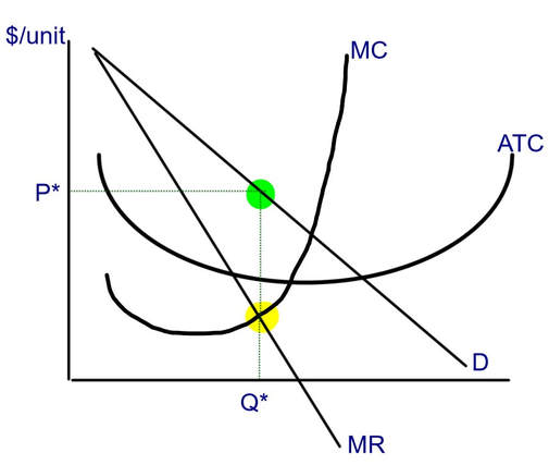
The monopolist chooses the profit-maximizing output level, Q*, by setting MR = MC (highlighted above in yellow). The firm then charges the price (P*) that people are willing to pay for this level of output (highlighted in green) as found on the demand curve.
Profit is found by finding the difference between the price that can be charged and the average total cost of production at the optimal quantity. Find the distance between the optimal price (on the demand curve) and the firm's average total cost curve. Multiply this by the optimal quantity:
Profit is found by finding the difference between the price that can be charged and the average total cost of production at the optimal quantity. Find the distance between the optimal price (on the demand curve) and the firm's average total cost curve. Multiply this by the optimal quantity:
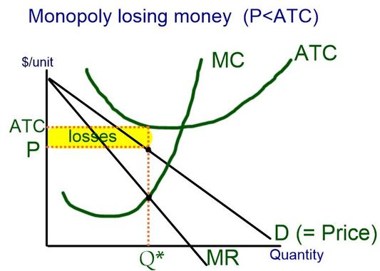
A monopolist can lose money if costs are high. The profit-maximizing output is still found by setting MR = MC; price is then chosen from the demand curve. (At any other output level / price, the firm would face larger losses). At the profit-maximizing output level of Q*, ATC is higher than Price and the firm loses money (since profit = Q x (P-ATC). The graph below illustrates this situation:
The monopoly decision using algebra:
For many, it is easier to use algebra to solve for the monopolist's optimal price and outcome combination than to use graphs. The key is to keep the important decision criteria in mind: (1) profit maximization occurs at the quantity where Marginal Revenue = Marginal Cost and (2) once it knows this optimal quantity, the monopolist chooses its price from the demand curve.
We'll work with the following equations:
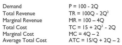
(The marginal revenue curve is twice as steep as the demand curve. Here, the slope of the MR curve is -4 while the slope of the demand curve is -2. The total revenue equation is the demand equation multiplied by quantity, since TR = P*Q. For those who know calculus, the MR curve is the first derivative of the Total Revenue curve and the Marginal Cost curve is the first derivative of the Total Cost curve).
We want to find the profit-maximizing output level, price, and the resulting profits (or loss).
Step 1: Find output (Q*) where MR = MC
MR = 100 - 4Q = 4Q – 2 = MC
100 + 2 = 4Q + 4Q
102 = 8Q
Q* = 102 / 8 = 12.75
Step 2: Find price (P*) using the demand curve equation
P* = 100 – 2Q* = 100 – 2(12.75) = 74.5
Step 3: Find profit as either TR – TC or as Q(P-ATC). The second equation is the fastest method since we already have Q and P. Find ATC by inserting Q* into the equation:
ATC = 15/Q + 2Q – 2 = 15/12.75 + 2(12.75) -2 = 1.17 + 25.5 - 2 = 24.67
π = Q x (P-ATC) = 12.75(74.5-24.67) = 12.75*49.83 = 635.33
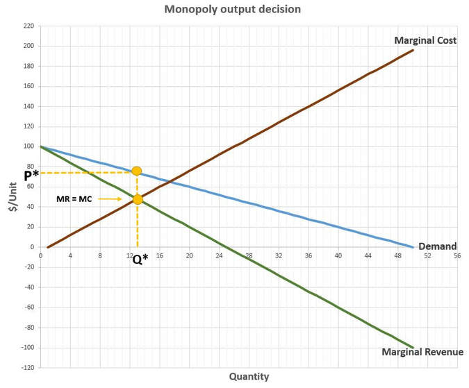
The graph of these equations confirms our analysis. (I've chosen not to show profit to highlight the first two steps):
We want to find the profit-maximizing output level, price, and the resulting profits (or loss).
Step 1: Find output (Q*) where MR = MC
MR = 100 - 4Q = 4Q – 2 = MC
100 + 2 = 4Q + 4Q
102 = 8Q
Q* = 102 / 8 = 12.75
Step 2: Find price (P*) using the demand curve equation
P* = 100 – 2Q* = 100 – 2(12.75) = 74.5
Step 3: Find profit as either TR – TC or as Q(P-ATC). The second equation is the fastest method since we already have Q and P. Find ATC by inserting Q* into the equation:
ATC = 15/Q + 2Q – 2 = 15/12.75 + 2(12.75) -2 = 1.17 + 25.5 - 2 = 24.67
π = Q x (P-ATC) = 12.75(74.5-24.67) = 12.75*49.83 = 635.33
The graph of these equations confirms our analysis. (I've chosen not to show profit to highlight the first two steps):
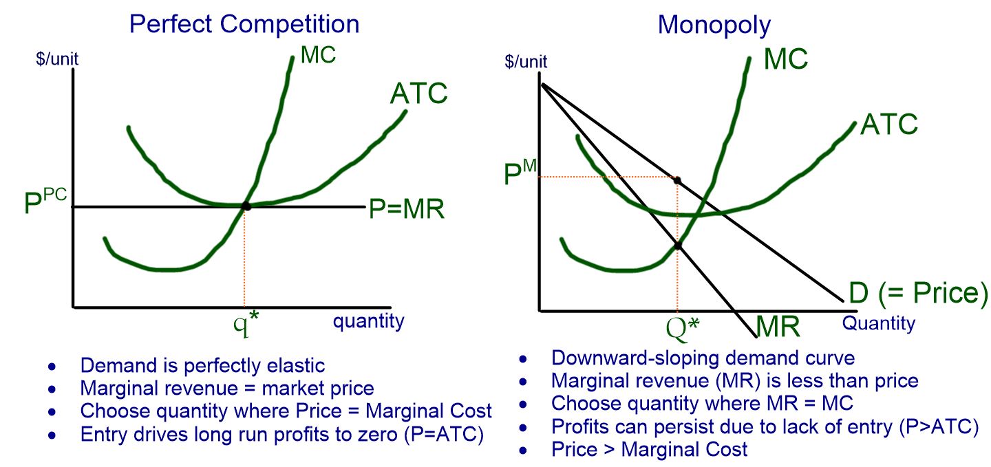
Monopoly vs. Perfect Competition
In the real world, true monopoly and perfect competition are pretty scarce. Nearly all firms face some kind of competition: the natural gas company in town must compete with the electric company (and with solar power). The owner of a patent for a cholesterol drug faces competition from companies with patents on different cholesterol drugs. Similarly, it is difficult to find a market that meets all of the requirements for perfect competition. In particular, we live in a world of product differentiation: firms produce products that are close but not perfect substitutes for each other. Nevertheless, knowing the expected outcomes from perfectly competitive and monopoly models helps us judge the impact of real-world competition. Is a business charging a price close to marginal cost? If so, it is producing near the perfectly competitive level. Conversely, a business that charges a price far above its marginal costs of production is judged to have a good deal of monopoly power.
In general, for firms facing similar cost structures, the price charged by a monopolist will be greater than the price charged by a perfectly competitive firm and the quantity produced by a monopolist will be lower than the quantity produced by a perfectly competitive firm. Consumers pay more for a lower quantity of output under a monopolist.
The graph below illustrates the perfect competition and monopoly decisions for firms with the same cost structure. Long run entry and exit drive price to the minimum of average total cost for firms in perfectly competitive markets and thus profits are zero. Profits persist for a monopolist as long as costs remain stable.
Sample problems for monopoly will be created soon!
Want to see these concepts demonstrated step-by-step? The following videos cover similar material (with the addition of price discrimination).
