Marginal Analysis and Profit Maximization
Dr. Amy McCormick Diduch
This section introduces one of the most powerful tools in microeconomics: marginal analysis. When describing decisions made by businesses or consumers, microeconomic models frequently focus on small incremental (or marginal) changes. The important conclusion of the model: the net benefits (or profits) of any activity are maximized when the marginal benefits received from the last step taken just equal the marginal costs of the last step.
Not all decisions are incremental! Big decisions require cost-benefit analysis, which compares the total costs and benefits of an activity to determine whether it should be pursued. Cost-benefit analysis may be used to determine whether a potential new environmental regulation is worth implementing or whether it is worthwhile for a business to build a new manufacturing facility. A complete cost-benefit analysis must take into account the direct costs and benefits of an action and the implicit costs and benefits (including the opportunity costs).
In many instances, the relevant decision is whether to increase or decrease an activity from some current level. A marginal change is a small change (an increase or decrease); this small change is likely to cause a change in the costs of an activity and a change in the benefits from the activity. Marginal analysis might be used by a business to determine the effects on profit of a change in the number of workers hired or a small change in output levels.
Important concepts for this analysis:
Total benefit (TB) is the sum of all benefits (direct and implicit) from pursuing an activity.
Marginal benefit (MB) is the change in total benefit from doing something once more (ΔTB / ΔQ).
Total cost (TC) is the sum of all costs (direct and implicit) from pursuing an activity.
Marginal cost (MC) is the change in total cost from doing something once more (ΔTC / ΔQ).
Net benefit (profit, π): Total benefit - total cost of a given action (TB – TC).
We assume that the goal of an individual or business is to maximize net benefit.
It is relatively easy to define total benefit for a business: this will include the total revenue from sales and any change in the value of assets for the business (the implicit revenue). Total costs include purchased materials and wages (the direct, or explicit, costs) as well as opportunity costs (for example, time spent training new employees or depreciation of capital equipment). For businesses, net benefit is defined as Profit (π) and calculated as Total Revenue (TR) – Total Cost (TC).
Defining total benefit for an individual is a bit more difficult. What is the total benefit to you of acquiring two pairs of shoes? How should we measure this? In practice, economists focus on an individual’s “willingness to pay” as an approximation of value. If you would be willing to pay $150 to acquire two pairs of shoes, the benefit of the shoes must be at least $150. In practice, this can be a difficult number to estimate, in part because what people are “willing to pay” varies by income level and because what they are “willing to accept” to give up an item is often significantly more than they say they would be “willing to pay” for it.
Suppose the table below reflects the total benefits an individual receives from having a given quantity of soccer shoes. Notice that if you have no shoes, you receive no benefit. Also, total benefit increases as the quantity of shoes increases. Although most models of consumer behavior assume this is true (i.e. that “more is better,”) it is not hard to imagine why you might not want to have 15 or 18 pairs of soccer shoes, even if they are given to you for free. If we extended this table, we might imagine that the 6th pair of soccer shoes is also worth $225 to you (so total benefit is not higher when you acquire another pair of shoes).
Marginal benefit (MB) is calculated as the change in Total Benefit divided by the change in Quantity (ΔTB / ΔQ). The third column shows the marginal benefit of acquiring one more pair of shoes. Quantity changes by 1 each time (so we are always dividing by 1 here):
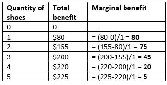
Marginal benefit is declining as the number of shoes owned increases. This table illustrates an important concept: diminishing marginal benefit.
Diminishing marginal benefit is likely to be present for most consumers and most goods. It might be easiest to understand if you think about it in the context of a favorite food. Having that first bite of chocolate adds a very large amount of benefit to chocolate lovers, but the 20th bite of chocolate probably adds much less to total benefit. Thus, the marginal benefits decline as the consumption of the good increases.
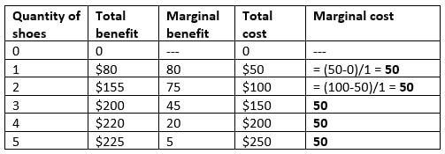
Assume that soccer shoes cost $50 a pair. (Yes, this is probably a bargain). We now add the total cost and marginal cost columns to our table. Notice that total cost here is just quantity of shoes multiplied by their price and marginal cost is equal to the price, since buying one more pair of shoes costs you $50.
Diminishing marginal benefit is likely to be present for most consumers and most goods. It might be easiest to understand if you think about it in the context of a favorite food. Having that first bite of chocolate adds a very large amount of benefit to chocolate lovers, but the 20th bite of chocolate probably adds much less to total benefit. Thus, the marginal benefits decline as the consumption of the good increases.
Assume that soccer shoes cost $50 a pair. (Yes, this is probably a bargain). We now add the total cost and marginal cost columns to our table. Notice that total cost here is just quantity of shoes multiplied by their price and marginal cost is equal to the price, since buying one more pair of shoes costs you $50.
We’ve assumed your goal is to maximize your net benefit. How many soccer shoes should you buy to achieve this goal? There are two ways to get the answer. First, we can directly calculate the net benefit of shoes for each quantity that you might purchase and pick the quantity of shoes for which this value is maximized.
Our second method is to use marginal analysis. We compare the marginal benefit and marginal cost of an action. Keep pursuing any action as long as the marginal benefits of doing so are greater than or equal to the marginal costs of the action. Why does this give us the right answer? Check the table above. The first pair of shoes adds $80 of benefits but only costs you $50. You should buy them. The second pair of shoes adds $75 to your benefits but only costs you $50. You should buy them. You place a value of $45 on the third pair of shoes but it costs you $50 to purchase them. You should not purchase the 3rd pair of shoes.
The table below adds the Net Benefit column and highlights the outcome from both methods. We calculate net benefit as (Total Benefit – Total Cost). This is maximized when you choose to buy 2 pairs of shoes.
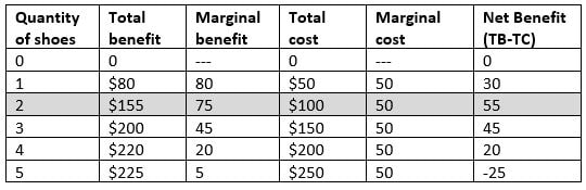
Notice that Net Benefit initially increases (the 2nd pair of shoes provides a higher net benefit than the 1st pair) before declining and eventually becoming negative (because having 5 pairs of shoes provides total benefits of $225 but costs $250).
Thus, we have two “rules of thumb” for decision making that will come to the same conclusion:
If we can measure small changes quite precisely, net benefits will be maximized where marginal benefit = marginal cost. (This is where calculus can help us, since the first derivative of an equation for total benefits or total costs provides us with the “marginal” change at a specific point. The marginal value is equal to the slope of the total benefit or cost function at a particular quantity).
Marginal analysis and business decisions:
Suppose the table below provides demand curve and cost information for a florist over a range of possible prices and quantities for floral arrangements. (The underlying demand equation used to generate the numbers here is P = 40 - .5QD and the underlying total cost equation is TC = 50 + 10Q). What should the business do if it wants to maximize profits?
Thus, we have two “rules of thumb” for decision making that will come to the same conclusion:
- The goal is to maximize net benefit of an activity. By calculating the difference between total benefits and total costs, we can determine which level will maximize net benefits.
- To maximize net benefit, continue the activity as long as Marginal Benefit ≥ Marginal Cost
If we can measure small changes quite precisely, net benefits will be maximized where marginal benefit = marginal cost. (This is where calculus can help us, since the first derivative of an equation for total benefits or total costs provides us with the “marginal” change at a specific point. The marginal value is equal to the slope of the total benefit or cost function at a particular quantity).
Marginal analysis and business decisions:
Suppose the table below provides demand curve and cost information for a florist over a range of possible prices and quantities for floral arrangements. (The underlying demand equation used to generate the numbers here is P = 40 - .5QD and the underlying total cost equation is TC = 50 + 10Q). What should the business do if it wants to maximize profits?
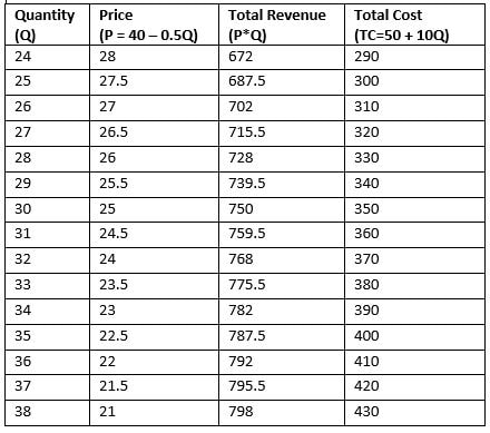
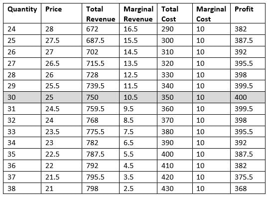
We can use either method to find the right answer. We can calculate net benefit, known here as profit (TR – TC) and choose the price and quantity combination that maximizes this. We can also calculate marginal benefit (here, it is called marginal revenue) and marginal cost, then recommend that the business choose the price and quantity combination at which marginal revenue equals marginal cost (or for which marginal revenue comes closest to marginal cost without exceeding it).
Here’s the full set of calculations:
Using the marginal rule:
Marginal Revenue is ∆TR/∆Q (or change in Total Revenue divided by change in Quantity), so the marginal revenue from increasing quantity from 24 to 25 is (687.5-672)/1 = 15.5.
Marginal Cost is ∆TC/∆Q (or change in Total Cost divided by change in Quantity), so the marginal cost from increasing quantity from 24 to 25 is (300 – 290)/1 = 10.
This company should increase output as long as the marginal revenue from doing so is greater than or equal to the marginal cost. Producing the 30th unit adds 10.5 to revenue and 10 to cost. It would not make sense to produce the 31st unit, for which the marginal revenue of 9.5 is less than the marginal cost incurred. Therefore, the firm maximizes profits by producing a quantity of 30 and charging a price of $25.
Maximizing net benefit:
Profit (π) is TR – TC. Thus, profit when quantity is 24 is 672-290 = 382.
Profit is maximized at a quantity of 30 and a price of $25. Total Revenue is 750, Total Cost is 350 and profit is $400.
We can convey the same information (and draw the same conclusions) using graphs. The most commonly used graphs in microeconomics illustrate the marginal benefit and marginal cost relationships (as shown in the graph on the far right). Visually, we can see that it is worth increasing an activity as long as the marginal benefit curve is above the marginal cost curve. The optimal quantity is where the marginal benefit curve crosses the marginal cost curve.
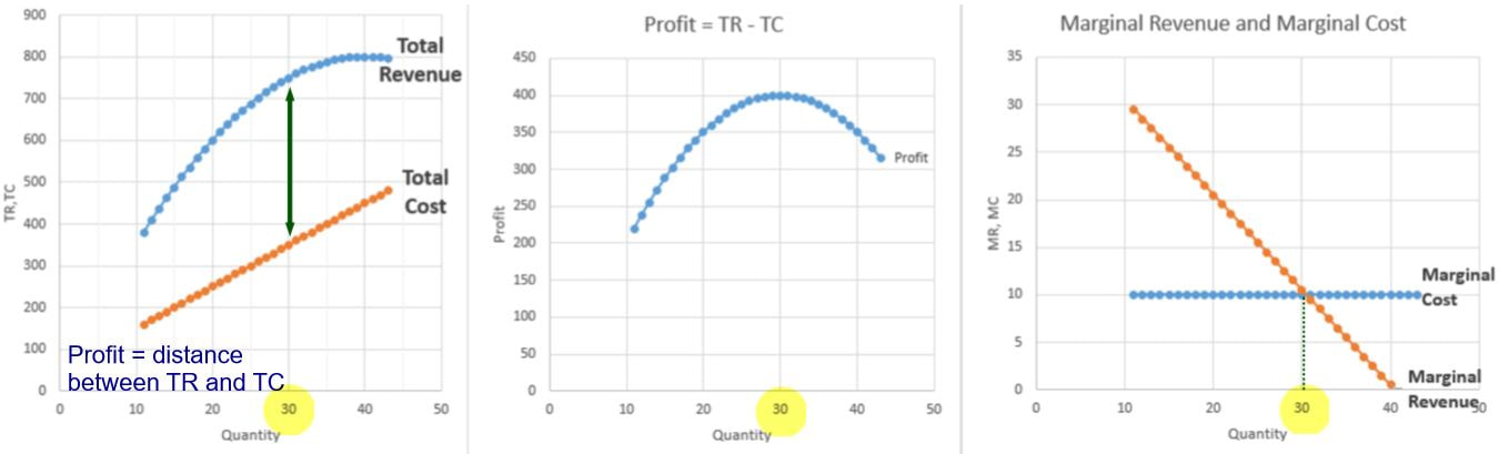
Math note:
If we know the linear demand relationship, we know that the marginal revenue relationship will have the same vertical intercept but will have twice the slope. The demand curve behind these numbers is P = 40 – 0.5Q. Thus, marginal revenue for this example is defined by the equation MR = 40 - QD. Marginal costs are constant at 10. We maximize net benefits by setting MR = MC (i.e. 40-Q = 10). This gives us the profit-maximizing quantity of 30 and, plugging this quantity into the original demand curve, a price of 25, which is the same answer we obtained in the table above. Using this linear equation to calculate the Marginal Revenue values in the table would produce slightly different numbers because it is more precise. Using this equation, we find that at a quantity of 30, MR = 10 and thus MR exactly equals MC at this quantity. In general, if we know the equation for demand, it is simpler to work with equations than with tables! However, if the demand equation is not linear, we do need to use calculus to find the marginal revenue curve (which is the first derivative of the demand curve).
Practice problems with marginal analysis are provided in the file below:
| marginal_analysis_practice_problems.pdf |
