Labor Demand and Short Run Production Costs
Dr. Amy McCormick Diduch
Concepts:
Short run production and the choice of inputs
Broadly speaking, firms face two major production-related decisions: (1) how much output to produce and (2) how to best produce that output. Both of these decisions rely on marginal analysis and both are constrained, in the short run, by choices previously made by the firm. The output decision is analyzed in the context of the market structure in which the firm operates (i.e. perfect competition, oligopoly, monopoly, or monopolistic competition); profit-maximizing firms in these models moslty choose the output level at which the marginal revenue from the last unit produced equals the marginal cost of producing it.
The short run production decision - discussed in this tutorial - comprises the choice of the optimal quantity of variable inputs such as labor, energy or raw materials. The long run production decision (not covered here) involves the introduction of new technology, the ultimate size of the business, and the mix of capital equipment and labor. The short run, therefore, is defined as the period of time in which certain production inputs are fixed. If the firm wants to increase or decrease output, it can do so only by changing its variable inputs. The long run, then, is the period of time in which the firm can change all of its inputs. There are no fixed inputs in the long run, only variable inputs. Most economic models assume that capital is fixed in the short run. It is certainly true that many firms cannot change the size of their production space or or the quantity of specialized equipment easily in the short run.
Profit-maximizing firms compare the marginal benefits of any choice with the marginal costs of that choice. Marginal analysis can be applied to the choice of inputs: hire more workers as long as their marginal benefit is greater than or equal to their marginal cost. How do we determine the marginal benefit of a worker? What is the marginal cost of hiring a worker?
Marginal revenue product
Firms hire workers because they want to sell the output produced by those workers. We describe labor demand as a derived demand since it is derived from the firm’s desire to produce a certain output level.
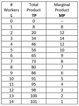
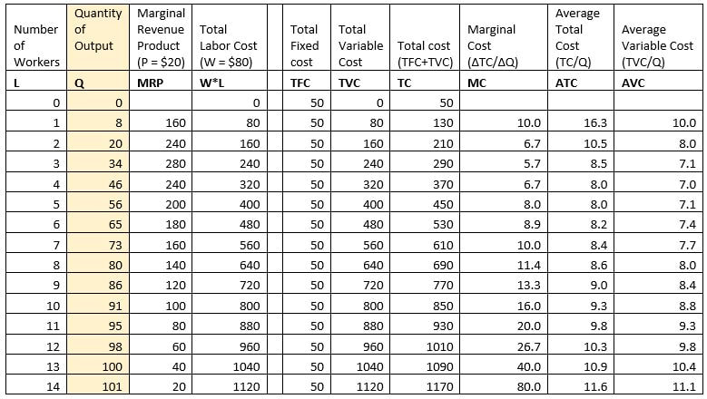
In choosing the optimal number of workers, a firm must estimate the total output level those workers are likely to produce. Total product refers to the output level associated with a specific quantity of workers. Marginal product measures the change in total product as a result of adding one more worker. Assume the table below contains data for a hypothetical pet grooming shop. The total product column records the number of pets that a given quantity of labor could groom in a day. The marginal product column records the impact on output of adding one more worker. For example, adding the 5th worker increases total product from 46 to 56 so the marginal product of the 5th worker is 10 extra pets groomed. Adding the 10th worker increases total product from 86 to 91 so the marginal product of the 10th worker is 5 extra pets groomed.
Dr. Amy McCormick Diduch
Concepts:
- Short run vs. long run production
- Total product and marginal product of labor
- Diminishing marginal product
- Marginal revenue product and the profit-maximizing choice of labor
- Impact of changes in price, marginal product, and wage on labor choice
- Costs of production in the short run and long run
Short run production and the choice of inputs
Broadly speaking, firms face two major production-related decisions: (1) how much output to produce and (2) how to best produce that output. Both of these decisions rely on marginal analysis and both are constrained, in the short run, by choices previously made by the firm. The output decision is analyzed in the context of the market structure in which the firm operates (i.e. perfect competition, oligopoly, monopoly, or monopolistic competition); profit-maximizing firms in these models moslty choose the output level at which the marginal revenue from the last unit produced equals the marginal cost of producing it.
The short run production decision - discussed in this tutorial - comprises the choice of the optimal quantity of variable inputs such as labor, energy or raw materials. The long run production decision (not covered here) involves the introduction of new technology, the ultimate size of the business, and the mix of capital equipment and labor. The short run, therefore, is defined as the period of time in which certain production inputs are fixed. If the firm wants to increase or decrease output, it can do so only by changing its variable inputs. The long run, then, is the period of time in which the firm can change all of its inputs. There are no fixed inputs in the long run, only variable inputs. Most economic models assume that capital is fixed in the short run. It is certainly true that many firms cannot change the size of their production space or or the quantity of specialized equipment easily in the short run.
Profit-maximizing firms compare the marginal benefits of any choice with the marginal costs of that choice. Marginal analysis can be applied to the choice of inputs: hire more workers as long as their marginal benefit is greater than or equal to their marginal cost. How do we determine the marginal benefit of a worker? What is the marginal cost of hiring a worker?
Marginal revenue product
Firms hire workers because they want to sell the output produced by those workers. We describe labor demand as a derived demand since it is derived from the firm’s desire to produce a certain output level.
In choosing the optimal number of workers, a firm must estimate the total output level those workers are likely to produce. Total product refers to the output level associated with a specific quantity of workers. Marginal product measures the change in total product as a result of adding one more worker. Assume the table below contains data for a hypothetical pet grooming shop. The total product column records the number of pets that a given quantity of labor could groom in a day. The marginal product column records the impact on output of adding one more worker. For example, adding the 5th worker increases total product from 46 to 56 so the marginal product of the 5th worker is 10 extra pets groomed. Adding the 10th worker increases total product from 86 to 91 so the marginal product of the 10th worker is 5 extra pets groomed.
Graphing the data from the table, we see that while total product increases as the number of workers increases, it does so in smaller and smaller increments. This is reflected in the downward-sloping marginal product of labor curve in the graph on the right. In fact, we expect most short run production processes to look like this. Why?
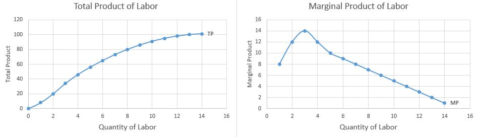
In the short run the firm has a fixed amount of space and a fixed amount of capital equipment. The first few workers may initially find ways of increasing their combined production quantities but eventually, as more and more workers are added, they will run into the problems of lack of space and lack of capital. The additional output obtained from adding each extra worker will get smaller and smaller. This problem is known as diminishing marginal product of labor and accouts for why the labor demand curve will slope downwards in the short run. It also accounts for the upward-sloping marginal cost curve faced by firms: in order to increase output in the short run, the firm must add increasingly larger amounts of labor to overcome the problem of diminishing marginal product.
A firm does benefit from hiring more workers, but the size of that benefit gets smaller with each new worker hired. The decision to hire – or not hire – another worker will depend on the value of the new output to the firm and the cost of hiring the worker.
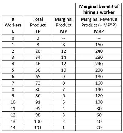
The value of the output produced by a worker is known as marginal revenue product (MRP) and can be calcluated as the price of the output multipled by the worker’s marginal product. In other words, it is the amount of revenue that is generated when the worker’s output is sold. (This value is sometimes termed the value of the marginal product or VMP).
Marginal Revenue Product = Marginal Product (MP) x Price
Assume that the price of pet grooming is $20. We can calculate the Marginal Revenue Product – the marginal benefit of hiring a worker - as follows:
A firm does benefit from hiring more workers, but the size of that benefit gets smaller with each new worker hired. The decision to hire – or not hire – another worker will depend on the value of the new output to the firm and the cost of hiring the worker.
The value of the output produced by a worker is known as marginal revenue product (MRP) and can be calcluated as the price of the output multipled by the worker’s marginal product. In other words, it is the amount of revenue that is generated when the worker’s output is sold. (This value is sometimes termed the value of the marginal product or VMP).
Marginal Revenue Product = Marginal Product (MP) x Price
Assume that the price of pet grooming is $20. We can calculate the Marginal Revenue Product – the marginal benefit of hiring a worker - as follows:
What is the marginal cost of hiring a worker? We will make several strong assumptions here. (If these assumptions do not hold, we’ll need to use a more complex model of labor demand). First, we assume that workers are identical and can be hired in the local labor market at a competitive wage. Second, we assume that this hourly wage is the primary cost of hiring workers (and thus can safely ignore the impact of benefits or training costs on the labor demand decision). For this simple model of labor demand, the wage is the marginal cost of hiring workers.
Assume the local wage is $80 per day. How many workers should the firm hire? Apply our tools of marginal analysis: hire workers up to the point where the marginal benefit (i.e. the marginal revenue product) just equals the marginal cost (i.e. the wage).
Short run labor demand: add workers as long as MRP ≥ wage
Based on the table above, this firm should hire 11 workers (who will groom 95 pets). Hiring the 12th worker would allow them to see three more pets per day but the extra revenue from those pets is only $60 and they would have to pay the 12th worker a wage of $80. The 11th worker produces $80 worth of output and is paid $80.
The graph of this marginal benefit – marginal cost decision is important. We graph only the downward-sloping portion of the marginal revenue product curve because a firm wouldn’t want to stop the hiring process at a point where adding new workers produces substantially more output compared to costs (as it could when the number of workers is very small). The marginal cost curve here is a horizontal line representing the local wage rate (since we have assumed that the firm can hire all the workers it wants at the current wage rate).
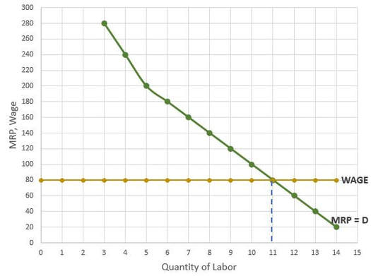
The marginal revenue product curve answers the question “how many workers should we hire if the wage is $X?” In other words, we can read the quantity of workers demanded at any “price” from the MRP curve. This means that the marginal revenue product curve is functioning as the firm’s labor demand curve. Thus, we’ve labeled the MRP curve as the Demand curve in the graph above.
This firm’s optimal quantity of labor will change if (1) the local wage rate changes, (2) the marginal product of workers changes or (3) the price of the firm’s output changes.
For example, at a daily wage of $100, this firm would choose to hire only 10 workers because the marginal benefit of the 11th worker is now less than the daily wage. If the local wage rate falls to $60, the firm will now hire 12 workers.
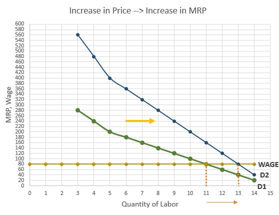
Suppose the price of pet grooming services increases to $40. What happens to the firm’s marginal revenue product curve and the optimal number of workers hired? We can recalculate the marginal revenue product values in the table and graph the new labor demand curve (labeled D2 in the graph below). When the price of pet grooming increases to $40, the firm wants to hire 13 workers because the value of the output produced by the 13th worker is now equal to the daily wage.
This firm’s optimal quantity of labor will change if (1) the local wage rate changes, (2) the marginal product of workers changes or (3) the price of the firm’s output changes.
For example, at a daily wage of $100, this firm would choose to hire only 10 workers because the marginal benefit of the 11th worker is now less than the daily wage. If the local wage rate falls to $60, the firm will now hire 12 workers.
Suppose the price of pet grooming services increases to $40. What happens to the firm’s marginal revenue product curve and the optimal number of workers hired? We can recalculate the marginal revenue product values in the table and graph the new labor demand curve (labeled D2 in the graph below). When the price of pet grooming increases to $40, the firm wants to hire 13 workers because the value of the output produced by the 13th worker is now equal to the daily wage.
Short run production and costs
Let’s consider the costs of running the pet grooming business described above. For simplicity, we’ll assume the firm uses two inputs: capital equipment and labor. (In reality, it also uses dog shampoos, water, electricity, etc. but we’ll ignore these other costs for the sake of simplicity. Adding them back in would not change our conclusions significantly). The cost of capital is fixed in the short run while labor is a variable cost that changes with the number of workers hired.
This table contains a lot of numbers! But if you take just a minute to look at the relationships between these figures, you’ll see patterns emerge.
First four columns: I’ve retained the production data for our pet grooming business and I’ve highlighted the output column. As we increase the number of workers hired, the quantity of output increases. The next column, marginal revenue product, assumes the original price of grooming services ($20). Total labor cost is calculated as the number of workers times the daily wage of $80. Thus, the daily cost of hiring 3 workers would be $240 (which is $80 x 3).
Total cost columns: The total cost columns record information about total fixed costs (here, $50 per day), total variable costs (here, the costs associated with hiring a given quantity of workers) and the total costs of producing a given quantity of output (which equals the sum of fixed and variable costs). Thus,
Total Cost = Total Variable Cost + Total Fixed Cost
Marginal and average cost columns:
Average Total Cost (ATC) = Average Variable Cost (AVC) + Average Fixed Cost (AFC)
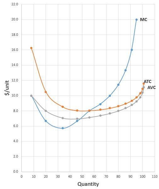
The marginal and average costs curves for the pet groomer are displayed in the graph below. The average total and average variable costs curves are roughly “U-shaped” and the marginal cost curve is roughly “J-shaped.” The average variable and average total cost curves are far apart when output is low but draw closer together as output increases. This is due to the declining importance of average fixed costs as output gets larger. (Why? We are dividing the same constant fixed cost value by a larger and larger amount of output).
The marginal cost curve crosses through the minimum points of the average varaible cost and average total cost curves. This is an important detail that will help you sketch these curves quickly!
Profit-maximizing output and quantity of labor
A profit-maximizing perfectly competitive firm will choose the output level for which Price = Marginal Cost and choose the quantity of labor for which MRP = Wage. Take a look at the table above! The price of pet grooming is $20. Setting P = MC, this firm would choose an output level of 95. To produce this output, the firm will hire 11 workers. The marginal revenue product of the 11th worker is just equal to the daily wage of $80. Thus, our marginal analysis holds for both the output level and the underlying labor demand.
- The marginal cost of production (MC) is the change in total cost resulting from a change in the quantity of output. To calculate Marginal Cost in this table, we need to divide the change in total cost (from the TC column) by the change in output (from the highlighted quantity of output column). Notice that Marginal Cost initially declines. This is where the marginal product of labor is increasing. However, Marginal Cost begins increasing after the 4th worker is hired and, in fact, increases quite sharply when the 13th and 14th workers are hired. This pattern of increasing marginal cost can be traced directly to the problem of diminishing marginal product of labor. Suppose we currently have 3 workers and we want to increase output by 10 units. We can do this (and more) by adding the 4th worker. Suppose we now have 8 workers and we want to increase output by 10 units. We would now need to add 2 workers if we want to increase output by 10.
- Average variable cost = Total variable cost / quantity and Average total cost = Total cost / quantity. I did not include a column for Average fixed cost (which equals Total fixed cost / quantity) because it does not tell us anything interesting about the production relationship (and because average fixed cost can be derived from the average total and average variable cost figures).
Average Total Cost (ATC) = Average Variable Cost (AVC) + Average Fixed Cost (AFC)
The marginal and average costs curves for the pet groomer are displayed in the graph below. The average total and average variable costs curves are roughly “U-shaped” and the marginal cost curve is roughly “J-shaped.” The average variable and average total cost curves are far apart when output is low but draw closer together as output increases. This is due to the declining importance of average fixed costs as output gets larger. (Why? We are dividing the same constant fixed cost value by a larger and larger amount of output).
The marginal cost curve crosses through the minimum points of the average varaible cost and average total cost curves. This is an important detail that will help you sketch these curves quickly!
Profit-maximizing output and quantity of labor
A profit-maximizing perfectly competitive firm will choose the output level for which Price = Marginal Cost and choose the quantity of labor for which MRP = Wage. Take a look at the table above! The price of pet grooming is $20. Setting P = MC, this firm would choose an output level of 95. To produce this output, the firm will hire 11 workers. The marginal revenue product of the 11th worker is just equal to the daily wage of $80. Thus, our marginal analysis holds for both the output level and the underlying labor demand.
The file below contains practice problems for this material.
| practice_problems_-_labor_demand_and_costs.pdf |
Want to see these concepts demonstrated step-by-step? The videos below cover this material in a similar format. The first video covers accounting profit vs. economic profit (not fully discussed in the written material above). The second video applies marginal analysis to labor demand and the third and fourth videos covers the full set of cost curves for the firm, including pointers on how to sketch them.
