
Production Possibilities Frontiers
Econ 101 Tutorial
Dr. Amy McCormick Diduch
Microeconomics is, in part, the study of how individuals, businesses and societies make choices in the face of scarcity. Choices arise because we do not have the resources (i.e. money, inputs or time) to acquire all of the good things we’d like to have or do, even when we are using our resources as efficiently as possible. Our first economic model – production possibilities – helps us illustrate the problems of scarcity and choice.
Production possibilities frontiers illustrate
To work with PPFs, you need to be able to do several things:
In this example, I’ll show you how to plot the points of the production possibility frontier (PPF), determine whether any given combination is inside, on, or outside the PPF, calculate opportunity cost, and shift the PPF to illustrate the impact of economic growth.
The PPF model is a simplified version of the real world. We consider an economy that produces only two goods (here, pies and sweaters, representing food and clothing). However, the insights from this simplified model are still relevant for our much more complex world.
Producing pies and sweaters requires resources: land, labor, physical capital, and management. Our maximum possible production of these goods depends on our access to these resources as well as the level of technology we have available. Moreover, if we devote all of our resources towards sweater production, we cannot produce any pies and if we devote all of our resources towards pie production, we cannot produce any sweaters. However, we can choose to divide our resources in ways that produce some of each.
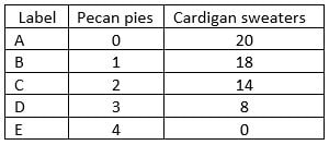
A production possibilities table lists possible output levels for our pies and sweaters. By definition, all of these combinations are “efficient” because they each represent ways of using our resources that produce the maximum combined output of these goods. According to this table, we can produce 20 sweaters if we devote all of our resources to sweater production. If we devote all of our resources to pie production, we can produce 4 pies. The remaining combinations listed in the table show how we can use our resources efficiently to produce some of both.
Although many of the insights of the PPF model can be gleaned from this table, it is often useful to plot this data onto a graph. Visualizing the PPF can help us understand the difference between attainable, efficient, and unattainable production combinations and understand the impact of technological change on the relative availability and prices of goods. For this example, we’ll graph pies on the horizontal axis (i.e. x-axis) and sweaters on the vertical axis (i.e. y-axis).
Step 1: plot the PPF
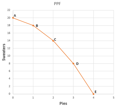
In the graph space below, I use the data in the table to plot each combination of pecan pies and cardigan sweaters. Each combination from the table is marked with its corresponding letter. For example, it is possible to produce a combination of 2 pies and 14 sweaters; letter “C” marks this combination. It is also possible to produce a combination of 0 pies and 20 sweaters; the letter “A” marks this combination. Note that I have labeled each axis (pies on the horizontal and sweaters on the vertical axis).
Econ 101 Tutorial
Dr. Amy McCormick Diduch
Microeconomics is, in part, the study of how individuals, businesses and societies make choices in the face of scarcity. Choices arise because we do not have the resources (i.e. money, inputs or time) to acquire all of the good things we’d like to have or do, even when we are using our resources as efficiently as possible. Our first economic model – production possibilities – helps us illustrate the problems of scarcity and choice.
Production possibilities frontiers illustrate
- opportunity cost (the net benefit of the best alternative not chosen)
- what it means to achieve production efficiency
- economic growth or decline
- the impact of technological change
To work with PPFs, you need to be able to do several things:
- plot points on a graph and read data from a graph
- calculate opportunity cost (as the slope of the PPF)
- illustrate a change in the position of the PPF curve (due to changes in resources or technological change)
In this example, I’ll show you how to plot the points of the production possibility frontier (PPF), determine whether any given combination is inside, on, or outside the PPF, calculate opportunity cost, and shift the PPF to illustrate the impact of economic growth.
The PPF model is a simplified version of the real world. We consider an economy that produces only two goods (here, pies and sweaters, representing food and clothing). However, the insights from this simplified model are still relevant for our much more complex world.
Producing pies and sweaters requires resources: land, labor, physical capital, and management. Our maximum possible production of these goods depends on our access to these resources as well as the level of technology we have available. Moreover, if we devote all of our resources towards sweater production, we cannot produce any pies and if we devote all of our resources towards pie production, we cannot produce any sweaters. However, we can choose to divide our resources in ways that produce some of each.
A production possibilities table lists possible output levels for our pies and sweaters. By definition, all of these combinations are “efficient” because they each represent ways of using our resources that produce the maximum combined output of these goods. According to this table, we can produce 20 sweaters if we devote all of our resources to sweater production. If we devote all of our resources to pie production, we can produce 4 pies. The remaining combinations listed in the table show how we can use our resources efficiently to produce some of both.
Although many of the insights of the PPF model can be gleaned from this table, it is often useful to plot this data onto a graph. Visualizing the PPF can help us understand the difference between attainable, efficient, and unattainable production combinations and understand the impact of technological change on the relative availability and prices of goods. For this example, we’ll graph pies on the horizontal axis (i.e. x-axis) and sweaters on the vertical axis (i.e. y-axis).
Step 1: plot the PPF
In the graph space below, I use the data in the table to plot each combination of pecan pies and cardigan sweaters. Each combination from the table is marked with its corresponding letter. For example, it is possible to produce a combination of 2 pies and 14 sweaters; letter “C” marks this combination. It is also possible to produce a combination of 0 pies and 20 sweaters; the letter “A” marks this combination. Note that I have labeled each axis (pies on the horizontal and sweaters on the vertical axis).
Step 2: Find efficient, inefficient and unattainable combinations.
Efficiency: Any combination of pies and sweaters that lies on this PPF is considered to be efficient. Points A, B, C, D, E (and any point in between) are all equally efficient. It is efficient to produce 0 pies and 20 sweaters. It is also efficient to produce 4 pies and 0 sweaters. It is equally efficient to produce 1 pie and 18 sweaters. Efficiency has nothing to do with whether a combination is desirable.
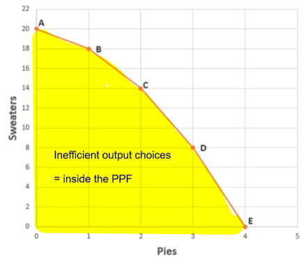
Inefficiency: For any given number of pies produced, if you produce less than the maximum possible number of sweaters, you are producing inefficiently. For example, if you are currently producing 3 pies and 6 sweaters, you are inefficient because you could have produced as many as 8 sweaters when producing 3 pies. In general, any combination of pies and sweaters that is “inside” the PPF is inefficient (represented by the yellow shading in the graph at right).
All of the choices along or inside of the PPF are attainable (i.e. society has the resources available to produce any of these combinations).
All of the choices along or inside of the PPF are attainable (i.e. society has the resources available to produce any of these combinations).
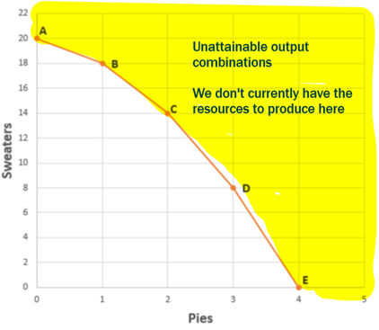
Unattainable:
Given your current resources, it is not possible to produce 4 pies and 14 sweaters. (Check your understanding by finding this combination in the graph at left: you'll see it is in the yellow shaded area). If you simply must have 4 pies, you’ll have to reduce the amount of sweaters to 0. If you simply must have 14 sweaters, you must reduce the amount of pies to 2. Any combination of pies and sweaters that is “outside” of the PPF is unattainable.
Step 3: Calculate the opportunity cost of pies in terms of sweaters given up.
How much does it cost to produce a pie? Cost is measured as opportunity cost: what you have to give up in order to get more pies. (The concept of opportunity cost works like a "cost / benefit" analysis: what must you sacrifice to get a particular gain?) We'll go back to our original table:
How much does it cost to produce a pie? Cost is measured as opportunity cost: what you have to give up in order to get more pies. (The concept of opportunity cost works like a "cost / benefit" analysis: what must you sacrifice to get a particular gain?) We'll go back to our original table:
Start at point A, where you have 0 pies and 20 sweaters. What do you have to give up in order to get 1 pie? You have to give up 2 sweaters (you have to reduce sweater production from 20 to 18).
Notice that the more pies you produce, the higher the cost in terms of sweaters forgone. This is an illustration of the law of increasing opportunity cost. A PPF will exhibit increasing opportunity cost any time resources are specialized, i.e. not perfectly suited to production of both goods. The graph of the PPF will be a curve when increasing opportunity costs are present. (If opportunity costs are constant, the PPF will be a straight line).
We expect most real-world production processes to exhibit increasing opportunity costs. Not all land is equally suitable for all production choices. Not all workers are equally skilled in producing all types of products. If we want to produce more and more of a particular kind of product (say, food), we will have to start converting resources better suited to production of other goods (such as clothing) into food production resources. This will become more and more difficult (i.e. costly).
Technical note: Calculating Opportunity Cost
Opportunity cost is defined here as the “loss of one good” in exchange for the “gain of another good” or (∆ quantity of lost good) divided by (∆ quantity of gained good) where ∆ means “change in”. In most of the examples in this tutorial we gain one unit of a good in exchange for increasing “losses” of another good so we are always dividing by 1. If the gain in pies was, say, 10 units each time, we would need to divide the loss of sweaters by the 10 pies gained. The final example in this tutorial shows you how to work with this.
Opportunity cost is essentially the slope of the production possibilities frontier. Slope is the change in the y-axis value divided by the change in the x-axis value or, in other words, the change in the quantity of the y-axis good in exchange for the change in the quantity of the x-axis good.
Technological change and the PPF
Technological change is the adoption of new methods of production that result in a higher level of output for a given level of inputs. Technological change can be “biased” – that is, affecting the production techniques in only one industry – or “unbiased” – affecting the production techniques in all industries.
“Biased” technological change
Suppose new technology significantly improves the production process for sweaters but the new technology does not directly improve the production of pecan pies. This “biased” technological change means that for any given amount of pie production, we can now produce more sweaters than before. The new production possibilities might look something like this:
- The cost of the first pie is 2 sweaters (calculated as 20-18).
- Notice that the cost of the second pie is 4 sweaters (you reduce sweater production from 18 to 14 in order to produce the 2nd pie so the opportunity cost is 18-14 = 4)
- The cost of the third pie is 6 sweaters (because you must reduce sweater production from 14 to 8).
- The cost of the fourth pie is 8 sweaters (because you must reduce sweater production from 8 to 0).
Notice that the more pies you produce, the higher the cost in terms of sweaters forgone. This is an illustration of the law of increasing opportunity cost. A PPF will exhibit increasing opportunity cost any time resources are specialized, i.e. not perfectly suited to production of both goods. The graph of the PPF will be a curve when increasing opportunity costs are present. (If opportunity costs are constant, the PPF will be a straight line).
We expect most real-world production processes to exhibit increasing opportunity costs. Not all land is equally suitable for all production choices. Not all workers are equally skilled in producing all types of products. If we want to produce more and more of a particular kind of product (say, food), we will have to start converting resources better suited to production of other goods (such as clothing) into food production resources. This will become more and more difficult (i.e. costly).
Technical note: Calculating Opportunity Cost
Opportunity cost is defined here as the “loss of one good” in exchange for the “gain of another good” or (∆ quantity of lost good) divided by (∆ quantity of gained good) where ∆ means “change in”. In most of the examples in this tutorial we gain one unit of a good in exchange for increasing “losses” of another good so we are always dividing by 1. If the gain in pies was, say, 10 units each time, we would need to divide the loss of sweaters by the 10 pies gained. The final example in this tutorial shows you how to work with this.
Opportunity cost is essentially the slope of the production possibilities frontier. Slope is the change in the y-axis value divided by the change in the x-axis value or, in other words, the change in the quantity of the y-axis good in exchange for the change in the quantity of the x-axis good.
Technological change and the PPF
Technological change is the adoption of new methods of production that result in a higher level of output for a given level of inputs. Technological change can be “biased” – that is, affecting the production techniques in only one industry – or “unbiased” – affecting the production techniques in all industries.
“Biased” technological change
Suppose new technology significantly improves the production process for sweaters but the new technology does not directly improve the production of pecan pies. This “biased” technological change means that for any given amount of pie production, we can now produce more sweaters than before. The new production possibilities might look something like this:
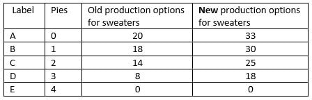
Nothing happens to the maximum possible production quantity of pies: if we use all of our resources to make pies, we still only get 4 pies. However, if we devote all of our resources to sweater production, we can now produce 33 sweaters rather than the 20 we previously produced.
The production possibilities frontier will rotate outward, as shown below. This graph shows both the original and the new PPFs. Any point on the new PPF is considered efficient. Any point inside of the new PPF (including our originally efficient points A, B, C and D) is attainable but inefficient. Thus, technological change helps us produce output combinations that were previously unattainable.
The production possibilities frontier will rotate outward, as shown below. This graph shows both the original and the new PPFs. Any point on the new PPF is considered efficient. Any point inside of the new PPF (including our originally efficient points A, B, C and D) is attainable but inefficient. Thus, technological change helps us produce output combinations that were previously unattainable.
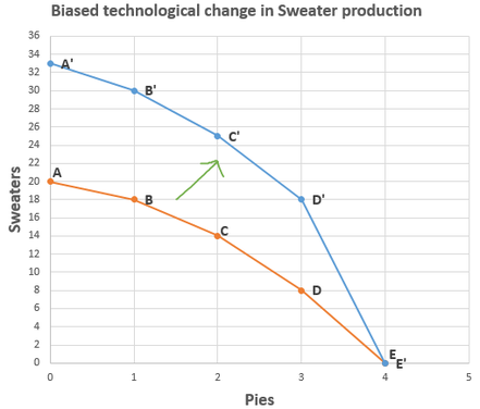
Suppose we were originally producing at point B (1 pie and 18 sweaters). Important insight: After this technological breakthrough in sweater production, we can now produce both more sweaters and more pies! For example, we might choose the new efficient point C’, at which we produce 2 pies and 25 sweaters. How can we increase pie production even if we only got technologically better at producing sweaters? Answer: we can transfer some of the resources previously used in sweater production into pie production.
Note that the law of increasing opportunity cost still holds. The “cost” of the first pie (moving from A to B) is 3 sweaters (since we have to reduce sweater production from 33 to 30); the cost of the second pie is 5 sweaters (= 30 -25), the cost of the third pie is 7 sweaters and the cost of the fourth pie is 18 sweaters.
Biased technological change and opportunity cost
Notice something very interesting: the “relative” cost of pies has increased and the “relative” cost of sweaters has decreased after this biased technological change! Since sweaters have become easier to produce (i.e. we can now produce more sweaters from any given amount of resources), we “give up” less to make sweaters than before. This means sweaters are relatively cheaper (and pies are relatively more expensive). Biased technological change affects real world tradeoffs! When manufactured goods become relatively cheaper to produce (as has happened over time worldwide), services (such as health care or education) now appear relatively more expensive to produce. This phenomenon is known as Baumol’s cost disease, named after economist William Baumol who first described it.
Other sources of economic growth: Unbiased technological change OR increase in quantity or quality of inputs
The entire production possibilities frontier may shift outward for one of three main reasons:
Note that the law of increasing opportunity cost still holds. The “cost” of the first pie (moving from A to B) is 3 sweaters (since we have to reduce sweater production from 33 to 30); the cost of the second pie is 5 sweaters (= 30 -25), the cost of the third pie is 7 sweaters and the cost of the fourth pie is 18 sweaters.
Biased technological change and opportunity cost
Notice something very interesting: the “relative” cost of pies has increased and the “relative” cost of sweaters has decreased after this biased technological change! Since sweaters have become easier to produce (i.e. we can now produce more sweaters from any given amount of resources), we “give up” less to make sweaters than before. This means sweaters are relatively cheaper (and pies are relatively more expensive). Biased technological change affects real world tradeoffs! When manufactured goods become relatively cheaper to produce (as has happened over time worldwide), services (such as health care or education) now appear relatively more expensive to produce. This phenomenon is known as Baumol’s cost disease, named after economist William Baumol who first described it.
Other sources of economic growth: Unbiased technological change OR increase in quantity or quality of inputs
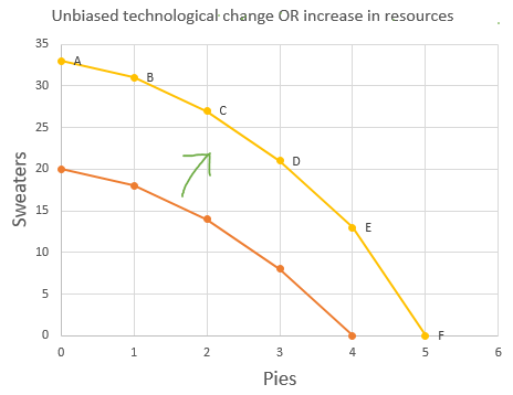
The entire production possibilities frontier may shift outward for one of three main reasons:
- There are more inputs available for production
- The quality of productive inputs increases
- “Unbiased” technological change improves our productive ability in both industries. (An example of unbiased technological change is the personal computer, which is used in almost every sector of the economy).
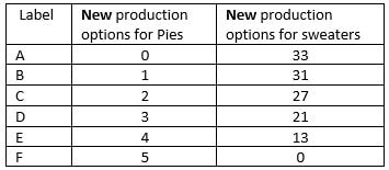
The new PPF still follows the law of increasing opportunity cost. The cost of the first pecan pie (moving from A to B) is 2 sweaters (reducing sweater production from 33 to 31). The cost of the second pie is 4 sweaters. The cost of the third pie is 6 sweaters. The cost of the fourth pie is 8 sweaters. The cost of the fifth pie is 13 sweaters.
When the PPF shifts outward, production choices that were previously unattainable are now attainable. For example, the new production choice C contains 27 sweaters and 2 pies. Before the shift this combination was unattainable but after the shift this combination is considered efficient.
When the PPF shifts outward, production choices that were previously unattainable are now attainable. For example, the new production choice C contains 27 sweaters and 2 pies. Before the shift this combination was unattainable but after the shift this combination is considered efficient.
More on calculating opportunity cost:
Opportunity cost along a PPF is calculated as (Loss in quantity of y-axis good) / (Gain in quantity of x-axis good)
Let’s calculate opportunity cost for a different set of production possibilities. Assume Cat toys are graphed on the x-axis and Dog toys on the Y-axis.
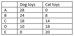
- Suppose we are currently producing at combination A. What is the opportunity cost of increasing production of cat toys? We lose 4 dog toys for the gain of 8 cat toys, so the cost “per” cat toy is 4 / 8 or ½.
- Suppose we are at combination C. What is the opportunity cost of increasing production of cat toys now? We lose 8 dog toys for a gain of 4 cat toys, so the “cost per cat toy” is 8 / 4 = 2.
- Suppose we are at combination D. What is the opportunity cost of increasing production of cat toys? We lose 10 dog toys for a gain of 2 cat toys, so the “cost per cat toy” is 10 / 2 = 5.
- Notice this PPF does exhibit increasing opportunity costs. We give up more and more dog toys in response to each attempt to increase production of cat toys.
Click on the PDF below it to download practice problems (with answers).
| production_possibilities_frontiers_practice_problems.pdf |
